Vincent Van Gogh painted this beautiful art: ‘The Starry Night’ in 1889 and today my GAN model (I like to call it GAN Gogh :P) painted some MNIST digits with only 20% labeled data!! How could it achieve this remarkable feat? … Let’s find out
Introduction
What is semi-supervised learning?
Most deep learning classifiers require a large amount of labeled samples to generalize well, but getting such data is an expensive and difficult process. To deal with this limitation Semi-supervised learning is presented, which is a class of techniques that make use of a morsel of labeled data along with a large amount of unlabeled data.Many machine-learning researchers have found that unlabeled data, when used in conjunction with a small amount of labeled data can produce considerable improvement in learning accuracy. GANs have shown a lot of potential in semi-supervised learning where the classifier can obtain a good performance with very few labeled data.
Background on GANs
GANs are members of deep generative models. They are particularly interesting because they don’t explicitly represent a probability distribution over the space where the data lies. Instead, they provide some way of interacting less directly with this probability distribution by drawing samples from it.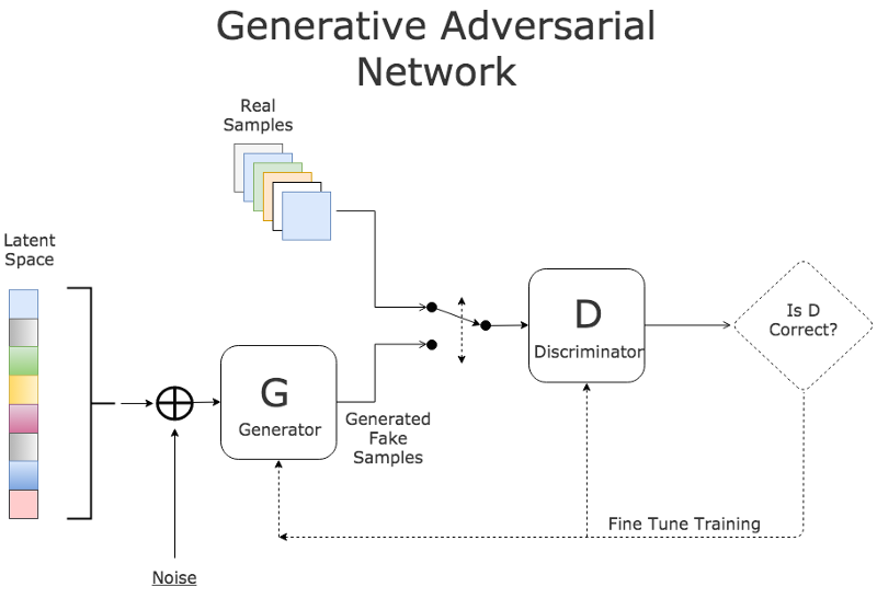
The basic idea of GAN is to set up a game between two players:
- A generator G: Takes random noise z as input and outputs an image x. Its parameters are tuned to get a high score from the discriminator on fake images that it generates.
- A discriminator D: Takes an image x as input and outputs a score which reflects its confidence that it is a real image. Its parameters are tuned to have a high score when it is fed by a real image, and a low score when a fake image is fed from the generator.
I suggest you to go through this and this for more details on their working and optimisation objectives. Now, let us turn the wheels a little and talk about one of the most prominent applications of GANs, semi-supervised learning.
Intuition
The vanilla architecture of discriminator has only one output neuron for classifying the R/F probabilities. We train both the networks simultaneously and discard the discriminator after the training as it was used only for improving the generator.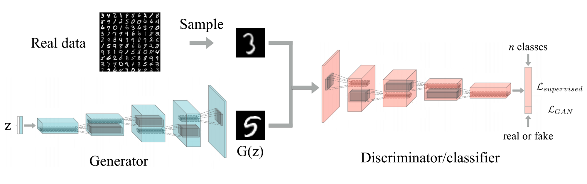
For the semi-supervised task, in addition to R/F neuron, the discriminator will now have 10 more neurons for classification of MNIST digits. Also, this time their roles change and we can discard the generator after training, whose only objective was to generate unlabeled data to improve the discriminator’s performance.
Now the discriminator is turned into an 11-class classifier with 1 neuron (R/F neuron) representing the fake data output and the other 10 representing real data with classes. The following has to be kept in mind:
- To assert R/F neuron output label = 0, when real unsupervised data from dataset is fed
- To assert R/F neuron output label= 1, when fake unsupervised data from generator is fed
- To assert R/F output label = 0 and corresponding label output = 1, when real supervised data is fed
This combination of different sources of data will help the discriminator classify more accurately than, if it had been only provided with a portion of labeled data.
Architecture
Now it’s time to get our hands dirty with some code :D
The Discriminator
The architecture followed is similar to the one proposed in DCGAN paper. We use strided convolutions for reducing the dimensions of the feature-vectors rather than any pooling layers and apply a series of leaky_relu, dropout and BN for all layers to stabilize the learning. BN is dropped for input layer and last layer (for the purpose of feature matching). In the end, we perform Global Average Pooling to take the average over the spatial dimensions of the feature vectors. This squashes the tensor dimensions to a single value. After flattening the features, a dense layer of 11 classes is added with softmax activation for multi-class output.1
2
3
4
5
6
7
8
9
10
11
12
13
14
15
16
17
18
19
20
21
22
23
24
25
26
27
28
29
30
31
32
33
34
35def discriminator(x, dropout_rate = 0., is_training = True, reuse = False):
# input x -> n+1 classes
with tf.variable_scope('Discriminator', reuse = reuse):
# x = ?*64*64*1
#Layer 1
conv1 = tf.layers.conv2d(x, 128, kernel_size = [4,4], strides = [2,2],
padding = 'same', activation = tf.nn.leaky_relu, name = 'conv1') # ?*32*32*128
#No batch-norm for input layer
dropout1 = tf.nn.dropout(conv1, dropout_rate)
#Layer2
conv2 = tf.layers.conv2d(dropout1, 256, kernel_size = [4,4], strides = [2,2],
padding = 'same', activation = tf.nn.leaky_relu, name = 'conv2') # ?*16*16*256
batch2 = tf.layers.batch_normalization(conv2, training = is_training)
dropout2 = tf.nn.dropout(batch2, dropout_rate)
#Layer3
conv3 = tf.layers.conv2d(dropout2, 512, kernel_size = [4,4], strides = [4,4],
padding = 'same', activation = tf.nn.leaky_relu, name = 'conv3') # ?*4*4*512
batch3 = tf.layers.batch_normalization(conv3, training = is_training)
dropout3 = tf.nn.dropout(batch3, dropout_rate)
# Layer 4
conv4 = tf.layers.conv2d(dropout3, 1024, kernel_size=[3,3], strides=[1,1],
padding='valid',activation = tf.nn.leaky_relu, name='conv4') # ?*2*2*1024
# No batch-norm as this layer's op will be used in feature matching loss
# No dropout as feature matching needs to be definite on logits
# Layer 5
# Note: Applying Global average pooling
flatten = tf.reduce_mean(conv4, axis = [1,2])
logits_D = tf.layers.dense(flatten, (1 + num_classes))
out_D = tf.nn.softmax(logits_D)
return flatten,logits_D,out_D
The Generator
The generator architecture is designed to mirror the discriminator’s spatial outputs. Fractional strided convolutions are used to increase the spatial dimension of the representation. An input of 4-D tensor of noise z is fed which undergoes a series of transposed convolutions, relu, BN(except at output layer) and dropout operations. Finally tanh activation maps the output image in range (-1,1).1
2
3
4
5
6
7
8
9
10
11
12
13
14
15
16
17
18
19
20
21
22
23
24
25
26
27
28
29
30def generator(z, dropout_rate = 0., is_training = True, reuse = False):
# input latent z -> image x
with tf.variable_scope('Generator', reuse = reuse):
#Layer 1
deconv1 = tf.layers.conv2d_transpose(z, 512, kernel_size = [4,4],
strides = [1,1], padding = 'valid',
activation = tf.nn.relu, name = 'deconv1') # ?*4*4*512
batch1 = tf.layers.batch_normalization(deconv1, training = is_training)
dropout1 = tf.nn.dropout(batch1, dropout_rate)
#Layer 2
deconv2 = tf.layers.conv2d_transpose(dropout1, 256, kernel_size = [4,4],
strides = [4,4], padding = 'same',
activation = tf.nn.relu, name = 'deconv2')# ?*16*16*256
batch2 = tf.layers.batch_normalization(deconv2, training = is_training)
dropout2 = tf.nn.dropout(batch2, dropout_rate)
#Layer 3
deconv3 = tf.layers.conv2d_transpose(dropout2, 128, kernel_size = [4,4],
strides = [2,2], padding = 'same',
activation = tf.nn.relu, name = 'deconv3')# ?*32*32*256
batch3 = tf.layers.batch_normalization(deconv3, training = is_training)
dropout3 = tf.nn.dropout(batch3, dropout_rate)
#Output layer
deconv4 = tf.layers.conv2d_transpose(dropout3, 1, kernel_size = [4,4],
strides = [2,2], padding = 'same',
activation = None, name = 'deconv4')# ?*64*64*1
out = tf.nn.tanh(deconv4)
return out
Model Loss
We start by preparing an extended label for the whole batch by appending actual label to zeros. This is done to assert the R/F neuron output to 0 when the labeled data is fed. The discriminator loss for unlabeled data can be thought of as a binary sigmoid loss by asserting R/F neuron output to 1 for fake images and 0 for real images.1
2
3
4
5
6
7
8
9
10
11
12
13
14
15
16
17
18
19 ### Discriminator loss ###
# Supervised loss -> which class the real data belongs to
temp = tf.nn.softmax_cross_entropy_with_logits_v2(logits = D_real_logit,
labels = extended_label)
# Labeled_mask and temp are of same size = batch_size where temp is softmax cross_entropy calculated over whole batch
D_L_Supervised = tf.reduce_sum(tf.multiply(temp,labeled_mask)) / tf.reduce_sum(labeled_mask)
# Multiplying temp with labeled_mask gives supervised loss on labeled_mask
# data only, calculating mean by dividing by no of labeled samples
# Unsupervised loss -> R/F
D_L_RealUnsupervised = tf.reduce_mean(tf.nn.sigmoid_cross_entropy_with_logits(
logits = D_real_logit[:, 0], labels = tf.zeros_like(D_real_logit[:, 0], dtype=tf.float32)))
D_L_FakeUnsupervised = tf.reduce_mean(tf.nn.sigmoid_cross_entropy_with_logits(
logits = D_fake_logit[:, 0], labels = tf.ones_like(D_fake_logit[:, 0], dtype=tf.float32)))
D_L = D_L_Supervised + D_L_RealUnsupervised + D_L_FakeUnsupervised
Generator loss is a combination of fake_image loss which falsely wants to assert R/F neuron output to 0 and feature matching loss which penalizes the mean absolute error between the average value of some set of features on the training data and the average values of that set of features on the generated samples.1
2
3
4
5
6
7
8
9
10
11
12 ### Generator loss ###
# G_L_1 -> Fake data wanna be real
G_L_1 = tf.reduce_mean(tf.nn.sigmoid_cross_entropy_with_logits(
logits = D_fake_logit[:, 0],labels = tf.zeros_like(D_fake_logit[:, 0], dtype=tf.float32)))
# G_L_2 -> Feature matching
data_moments = tf.reduce_mean(D_real_features, axis = 0)
sample_moments = tf.reduce_mean(D_fake_features, axis = 0)
G_L_2 = tf.reduce_mean(tf.square(data_moments-sample_moments))
G_L = G_L_1 + G_L_2
Training
The training images are resized from [batch_size, 28 ,28 , 1] to [batch_size, 64, 64, 1] to fit the generator/discriminator architectures. Losses, accuracies and generated samples are calculated and are observed to improve over each epoch.1
2
3
4
5
6
7
8
9
10
11
12
13
14
15
16
17
18
19
20
21
22
23
24
25
26
27
28
29
30
31
32
33
34
35
36
37
38for epoch in range(epochs):
train_accuracies, train_D_losses, train_G_losses = [], [], []
for it in range(no_of_batches):
batch = mnist_data.train.next_batch(batch_size, shuffle = False)
# batch[0] has shape: batch_size*28*28*1
batch_reshaped = tf.image.resize_images(batch[0], [64, 64]).eval()
# Reshaping the whole batch into batch_size*64*64*1 for disc/gen architecture
batch_z = np.random.normal(0, 1, (batch_size, 1, 1, latent))
mask = get_labeled_mask(labeled_rate, batch_size)
train_feed_dict = {x : scale(batch_reshaped), z : batch_z,
label : batch[1], labeled_mask : mask,
dropout_rate : 0.7, is_training : True}
#The label provided in dict are one hot encoded in 10 classes
D_optimizer.run(feed_dict = train_feed_dict)
G_optimizer.run(feed_dict = train_feed_dict)
train_D_loss = D_L.eval(feed_dict = train_feed_dict)
train_G_loss = G_L.eval(feed_dict = train_feed_dict)
train_accuracy = accuracy.eval(feed_dict = train_feed_dict)
train_D_losses.append(train_D_loss)
train_G_losses.append(train_G_loss)
train_accuracies.append(train_accuracy)
tr_GL = np.mean(train_G_losses)
tr_DL = np.mean(train_D_losses)
tr_acc = np.mean(train_accuracies)
print ('After epoch: '+ str(epoch+1) + ' Generator loss: '
+ str(tr_GL) + ' Discriminator loss: ' + str(tr_DL) + ' Accuracy: ' + str(tr_acc))
gen_samples = fake_data.eval(feed_dict = {z : np.random.normal(0, 1, (25, 1, 1, latent)), dropout_rate : 0.7, is_training : False})
# Dont train batch-norm while plotting => is_training = False
test_images = tf.image.resize_images(gen_samples, [64, 64]).eval()
show_result(test_images, (epoch + 1), show = True, save = False, path = '')
Conclusion
The training was done for 5 epochs and 20% labeled_rate due to restricted GPU access. For better results more training epochs with lesser labeled_rate is advised. The complete code notebook can be found here.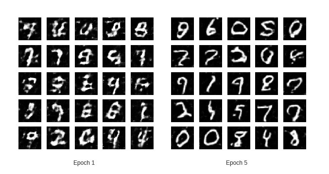
Unsupervised learning is considered as a lacuna in the field of AGI. To bridge this gap, GANs are considered as a potential solution for learning complex tasks with low labeled data. With blooming new approaches in the domain of semi and unsupervised learning we can expect that this gap will lessen.
I would be remiss not to mention my inspiration from this beautiful blog, this implementation along with the assistance of my colleague working on similar projects.
Until next time!! Kz