TensorFlowSharp安装和使用入门
(posted @ 2017-11-25 21:31)
Tensorflow是一个人工智能框架。TensorflowSharp是对Tensorflow C语言版接口的封装,便于C#开发人员在项目中使用Tensorflow。
一、使用方法
TensorflowSharp的使用很简单,首先使用NuGet安装TensorflowSharp包,然后新建C#控制台程序,输入下面代码,运行即可。1
2
3
4
5
6
7
8
9
10
11
12
13
14
15
16
17
18
19
20
21
22
23
24// 创建图
var g = new TFGraph();
// 定义常量
var a = g.Const(2);
var b = g.Const(3);
// 加法和乘法运算
var add = g.Add(a, b);
var mul = g.Mul(a, b);
// 创建会话
var sess = new TFSession(g);
// 计算加法
var result1 = sess.GetRunner().Run(add).GetValue();
Console.WriteLine("a+b={0}", result1);
// 计算乘法
var result2 = sess.GetRunner().Run(mul).GetValue();
Console.WriteLine("a*b={0}", result2);
// 关闭会话
sess.CloseSession();
运行后输出结果:1
2a+b=5
a*b=6
二、注意事项
- 国内目前无法访问Tensorflow官网,但是可以访问谷歌提供的Tensorflow官网镜像。
- 国内使用NuGet安装TensorflowSharp很容易失败,可以直接从Nuget官网下载,然后改后缀名zip,解压后手工安装。
- TensorflowSharp项目使用的.net版本必须高于4.6.1,本教程使用的版本是4.7.0,可以在属性选项卡中设置。
- TensorflowSharp项目必须使用64位CPU,需要在属性选项卡生成中,去掉首选32位的勾选。
- 手动安装TensorflowSharp,处理要引用TensorFlowSharp.dll,还要将libtensorflow.dll复制到每个项目的输出目录。
三、相关网站
Tensorflow教程:https://github.com/tengge1/learn-tensorflow-sharp
Tensorflow官网:http://www.tensorflow.org
Google Tensorflow镜像:https://tensorflow.google.cn/
Tensorflow开源项目:https://github.com/tensorflow/tensorflow
TensorflowSharp开源项目:https://github.com/migueldeicaza/TensorFlowSharp
TensorflowSharp NuGet主页:https://www.nuget.org/packages/TensorFlowSharp/
Tensorflow中文社区:http://www.tensorfly.cn/
03 使用TensorFlow做计算题
我们使用Tensorflow,计算((a+b)*c)^2/a,然后求平方根。看代码:1
2
3
4
5
6
7
8
9
10
11
12
13
14
15
16
17
18
19
20
21
22
23
24
25
26
27
28import tensorflow as tf
# 输入储存容器
a = tf.placeholder(tf.float16)
b = tf.placeholder(tf.float16)
c = tf.placeholder(tf.float16)
# 计算
d = tf.add(a, b) #加法
e = tf.multiply(d, c) #乘法
f = tf.pow(e, 2) #平方
g = tf.divide(f, a) #除法
h = tf.sqrt(g) #平方根
# 会话
sess = tf.Session()
# 赋值
feed_dict= {a:1, b:2, c:3}
# 计算
result = sess.run(h, feed_dict= feed_dict)
# 关闭会话
sess.close()
# 输出结果
print(result)
这里让a=1,b=2,c=3,如果输出9.0,证明运行成功。
Tensorflow做计算的方法是,先把计算的式子构建一个图,然后把这个图和赋值在cpu上一起运行,计算速度比较快。
04 TensorFlow中的常量、变量和数据类型
打开Python Shell,先输入import tensorflow as tf,然后可以执行以下命令。
Tensorflow中的常量创建方法:1
hello = tf.constant('Hello,world!', dtype=tf.string)
其中,’Hello,world!’是常量初始值;tf.string是常量类型,可以省略。常量和变量都可以去构建Tensorflow中的图。
Tensorflow中变量的创建方法:1
a = tf.Variable(10, dtype=tf.int32)
其中,10是变量初始值,tf.int32是变量的类型。
Tensorflow中,主要有以下几种数据类型。
tf.int8:8位整数。
tf.int16:16位整数。
tf.int32:32位整数。
tf.int64:64位整数。
tf.uint8:8位无符号整数。
tf.uint16:16位无符号整数。
tf.float16:16位浮点数。
tf.float32:32位浮点数。
tf.float64:64位浮点数。
tf.double:等同于tf.float64。
tf.string:字符串。
tf.bool:布尔型。
tf.complex64:64位复数。
tf.complex128:128位复数。
参考文献
05 TensorFlow中变量的初始化
打开Python Shell,输入import tensorflow as tf,然后可以执行以下代码。
1、创建一个2*3的矩阵,并让所有元素的值为0.(类型为tf.float)1
a = tf.zeros([2,3], dtype = tf.float32)
2、创建一个3*4的矩阵,并让所有元素的值为1.1
b = tf.ones([3,4])
3、创建一个1*10的矩阵,使用2来填充。(类型为tf.int32,可忽略)1
c = tf.constant(2, dtype=tf.int32, shape=[1,10])
4、创建一个1*10的矩阵,其中的元素符合正态分布,平均值是20,标准偏差是3.1
d = tf.random_normal([1,10],mean = 20, stddev = 3)
上面所有的值都可以用来初始化变量。例如用0.01来填充一个1*2的矩阵来初始化一个叫bias的变量。1
bias = tf.Variable(tf.zeros([1,2]) + 0.01)
如果你想查看这些量具体的值,可以在Session中执行它并输出。1
2sess = tf.Session()
print(sess.run(d))
这里,我得到了以下的值:
[[ 22.44503784 18.19544983 17.89671898 17.67314911 19.45074844
18.6805439 18.56541443 16.59041977 22.11240005 19.12819099]]。它就是上面4我们创建的量的值。
参考文献
06 使用TensorFlow拟合x与y之间的关系
看代码:1
2
3
4
5
6
7
8
9
10
11
12
13
14
15
16
17
18
19
20
21
22
23
24
25
26
27
28
29
30
31
32
33
34
35
36
37
38import tensorflow as tf
import numpy as np
#构造输入数据(我们用神经网络拟合x_data和y_data之间的关系)
x_data = np.linspace(-1,1,300)[:, np.newaxis] #-1到1等分300份形成的二维矩阵
noise = np.random.normal(0,0.05, x_data.shape) #噪音,形状同x_data在0-0.05符合正态分布的小数
y_data = np.square(x_data)-0.5+noise #x_data平方,减0.05,再加噪音值
#输入层(1个神经元)
xs = tf.placeholder(tf.float32, [None, 1]) #占位符,None表示n*1维矩阵,其中n不确定
ys = tf.placeholder(tf.float32, [None, 1]) #占位符,None表示n*1维矩阵,其中n不确定
#隐层(10个神经元)
W1 = tf.Variable(tf.random_normal([1,10])) #权重,1*10的矩阵,并用符合正态分布的随机数填充
b1 = tf.Variable(tf.zeros([1,10])+0.1) #偏置,1*10的矩阵,使用0.1填充
Wx_plus_b1 = tf.matmul(xs,W1) + b1 #矩阵xs和W1相乘,然后加上偏置
output1 = tf.nn.relu(Wx_plus_b1) #激活函数使用tf.nn.relu
#输出层(1个神经元)
W2 = tf.Variable(tf.random_normal([10,1]))
b2 = tf.Variable(tf.zeros([1,1])+0.1)
Wx_plus_b2 = tf.matmul(output1,W2) + b2
output2 = Wx_plus_b2
#损失
loss = tf.reduce_mean(tf.reduce_sum(tf.square(ys-output2),reduction_indices=[1])) #在第一维上,偏差平方后求和,再求平均值,来计算损失
train_step = tf.train.GradientDescentOptimizer(0.1).minimize(loss) # 使用梯度下降法,设置步长0.1,来最小化损失
#初始化
init = tf.global_variables_initializer() #初始化所有变量
sess = tf.Session()
sess.run(init) #变量初始化
#训练
for i in range(1000): #训练1000次
_,loss_value = sess.run([train_step,loss],feed_dict={xs:x_data,ys:y_data}) #进行梯度下降运算,并计算每一步的损失
if(i%50==0):
print(loss_value) # 每50步输出一次损失
输出:
0.405348
0.00954485
0.0068925
0.00551958
0.00471453
0.00425206
0.00400382
0.00381883
0.00367445
0.00353349
0.00341325
0.00330487
0.00321128
0.00313468
0.0030646
0.0030014
0.00294802
0.00290179
0.0028618
0.00282344
可以看到,随机训练的进行,损失越来越小,证明拟合越来越好。
参考文献
07 训练TensorFlow识别手写数字
打开Python Shell,输入以下代码:1
2
3
4
5
6
7
8
9
10
11
12
13
14
15
16
17
18
19
20
21
22
23
24
25
26
27
28
29
30
31
32
33
34import tensorflow as tf
from tensorflow.examples.tutorials.mnist import input_data
# 获取数据(如果存在就读取,不存在就下载完再读取)
mnist = input_data.read_data_sets("MNIST_data/", one_hot=True)
# 输入
x = tf.placeholder("float", [None, 784]) #输入占位符(每张手写数字784个像素点)
y_ = tf.placeholder("float", [None,10]) #输入占位符(这张手写数字具体代表的值,0-9对应矩阵的10个位置)
# 计算分类softmax会将xW+b分成10类,对应0-9
W = tf.Variable(tf.zeros([784,10])) #权重
b = tf.Variable(tf.zeros([10])) #偏置
y = tf.nn.softmax(tf.matmul(x,W) + b) # 输入矩阵x与权重矩阵W相乘,加上偏置矩阵b,然后求softmax(sigmoid函数升级版,可以分成多类)
# 计算偏差和
cross_entropy = -tf.reduce_sum(y_*tf.log(y))
# 使用梯度下降法(步长0.01),来使偏差和最小
train_step = tf.train.GradientDescentOptimizer(0.01).minimize(cross_entropy)
# 初始化变量
init = tf.global_variables_initializer()
sess = tf.Session()
sess.run(init)
for i in range(10): # 训练10次
batch_xs, batch_ys = mnist.train.next_batch(100) # 随机取100个手写数字图片
sess.run(train_step, feed_dict={x: batch_xs, y_: batch_ys}) # 执行梯度下降算法,输入值x:batch_xs,输入值y:batch_ys
# 计算训练精度
correct_prediction = tf.equal(tf.argmax(y,1), tf.argmax(y_,1))
accuracy = tf.reduce_mean(tf.cast(correct_prediction, "float"))
print(sess.run(accuracy, feed_dict={x: mnist.test.images, y_: mnist.test.labels})) #运行精度图,x和y_从测试手写图片中取值
执行该段代码,输出0.8002。训练10次得到80.02%的识别准确度,还是可以的。
说明:由于网络原因,手写数字图片可能无法下载,可以直接下载本人做好的程序,里面已经包含了手写图片资源和py脚本。(链接已失效)
参考文献
10 TensorFlow中模型保存与读取
我们的模型训练出来想给别人用,或者是我今天训练不完,明天想接着训练,怎么办?这就需要模型的保存与读取。看代码:1
2
3
4
5
6
7
8
9
10
11
12
13
14
15
16
17
18
19
20
21
22
23
24
25
26
27
28
29
30
31
32
33
34
35
36
37
38
39
40
41
42
43
44
45
46
47
48
49
50import tensorflow as tf
import numpy as np
import os
#输入数据
x_data = np.linspace(-1,1,300)[:, np.newaxis]
noise = np.random.normal(0,0.05, x_data.shape)
y_data = np.square(x_data)-0.5+noise
#输入层
xs = tf.placeholder(tf.float32, [None, 1])
ys = tf.placeholder(tf.float32, [None, 1])
#隐层
W1 = tf.Variable(tf.random_normal([1,10]))
b1 = tf.Variable(tf.zeros([1,10])+0.1)
Wx_plus_b1 = tf.matmul(xs,W1) + b1
output1 = tf.nn.relu(Wx_plus_b1)
#输出层
W2 = tf.Variable(tf.random_normal([10,1]))
b2 = tf.Variable(tf.zeros([1,1])+0.1)
Wx_plus_b2 = tf.matmul(output1,W2) + b2
output2 = Wx_plus_b2
#损失
loss = tf.reduce_mean(tf.reduce_sum(tf.square(ys-output2),reduction_indices=[1]))
train_step = tf.train.GradientDescentOptimizer(0.1).minimize(loss)
#模型保存加载工具
saver = tf.train.Saver()
#判断模型保存路径是否存在,不存在就创建
if not os.path.exists('tmp/'):
os.mkdir('tmp/')
#初始化
sess = tf.Session()
if os.path.exists('tmp/checkpoint'): #判断模型是否存在
saver.restore(sess, 'tmp/model.ckpt') #存在就从模型中恢复变量
else:
init = tf.global_variables_initializer() #不存在就初始化变量
sess.run(init)
#训练
for i in range(1000):
_,loss_value = sess.run([train_step,loss], feed_dict={xs:x_data,ys:y_data})
if(i%50==0): #每50次保存一次模型
save_path = saver.save(sess, 'tmp/model.ckpt') #保存模型到tmp/model.ckpt,注意一定要有一层文件夹,否则保存不成功!!!
print("模型保存:%s 当前训练损失:%s"%(save_path, loss_value))
大家第一次训练得到:
模型保存:tmp/model.ckpt 当前训练损失:1.35421
模型保存:tmp/model.ckpt 当前训练损失:0.011808
模型保存:tmp/model.ckpt 当前训练损失:0.00916655
模型保存:tmp/model.ckpt 当前训练损失:0.00690887
模型保存:tmp/model.ckpt 当前训练损失:0.00575491
模型保存:tmp/model.ckpt 当前训练损失:0.00526401
模型保存:tmp/model.ckpt 当前训练损失:0.00498503
模型保存:tmp/model.ckpt 当前训练损失:0.00478226
模型保存:tmp/model.ckpt 当前训练损失:0.0046346
模型保存:tmp/model.ckpt 当前训练损失:0.00454276
模型保存:tmp/model.ckpt 当前训练损失:0.00446402
模型保存:tmp/model.ckpt 当前训练损失:0.00436883
模型保存:tmp/model.ckpt 当前训练损失:0.00427732
模型保存:tmp/model.ckpt 当前训练损失:0.00418589
模型保存:tmp/model.ckpt 当前训练损失:0.00409241
模型保存:tmp/model.ckpt 当前训练损失:0.00400956
模型保存:tmp/model.ckpt 当前训练损失:0.00392799
模型保存:tmp/model.ckpt 当前训练损失:0.00383506
模型保存:tmp/model.ckpt 当前训练损失:0.00373741
模型保存:tmp/model.ckpt 当前训练损失:0.00366922
第二次继续训练,得到:
模型保存:tmp/model.ckpt 当前训练损失:0.00412003
模型保存:tmp/model.ckpt 当前训练损失:0.00388735
模型保存:tmp/model.ckpt 当前训练损失:0.00382827
模型保存:tmp/model.ckpt 当前训练损失:0.00379988
模型保存:tmp/model.ckpt 当前训练损失:0.00378107
模型保存:tmp/model.ckpt 当前训练损失:0.003764
模型保存:tmp/model.ckpt 当前训练损失:0.00375149
模型保存:tmp/model.ckpt 当前训练损失:0.00374324
模型保存:tmp/model.ckpt 当前训练损失:0.00373386
模型保存:tmp/model.ckpt 当前训练损失:0.00372364
模型保存:tmp/model.ckpt 当前训练损失:0.00371543
模型保存:tmp/model.ckpt 当前训练损失:0.00370875
模型保存:tmp/model.ckpt 当前训练损失:0.00370262
模型保存:tmp/model.ckpt 当前训练损失:0.00369697
模型保存:tmp/model.ckpt 当前训练损失:0.00369161
模型保存:tmp/model.ckpt 当前训练损失:0.00368653
模型保存:tmp/model.ckpt 当前训练损失:0.00368169
模型保存:tmp/model.ckpt 当前训练损失:0.00367714
模型保存:tmp/model.ckpt 当前训练损失:0.00367274
模型保存:tmp/model.ckpt 当前训练损失:0.00366843
可以看到,第二次训练是在第一次训练的基础上继续训练的。于是,我们可以把我们想要的模型保存下来,慢慢训练。
参考文献
- 《TensorFlow使用指南》:http://www.tensorfly.cn/tfdoc/tutorials/mnist_tf.html
- TensorFlow中模型保存与读取:https://www.cnblogs.com/tengge/p/6379893.html
11 使用TensorBoard显示图片
首先,下载一张png格式的图片(注意:只支持png格式),命名为1.png。然后,打开PythonShell,输入以下代码:1
2
3
4
5
6
7
8
9
10
11
12
13
14
15
16
17
18
19
20
21
22
23import tensorflow as tf
# 获取图片数据
file = open('1.png', 'rb')
data = file.read()
file.close()
# 图片处理
image = tf.image.decode_png(data, channels=4)
image = tf.expand_dims(image, 0)
# 添加到日志中
sess = tf.Session()
writer = tf.summary.FileWriter('logs')
summary_op = tf.summary.image("image1", image)
# 运行并写入日志
summary = sess.run(summary_op)
writer.add_summary(summary)
# 关闭
writer.close()
sess.close()
然后,在相同目录打开cmd,输入tensorboard —logdir=logs,然后打开浏览器输入http://localhost:6006/。在Tensorboard的Images标签页,就可以看到我们的png图片了。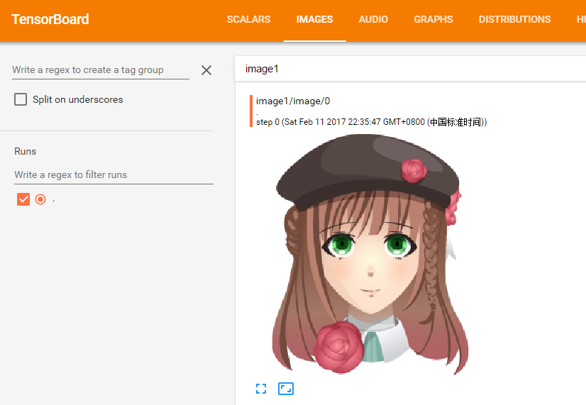
参考文献
12 使用卷积神经网络识别手写数字
看代码:1
2
3
4
5
6
7
8
9
10
11
12
13
14
15
16
17
18
19
20
21
22
23
24
25
26
27
28
29
30
31
32
33
34
35
36
37
38
39
40
41
42
43
44
45
46
47
48
49
50
51
52
53
54
55
56
57
58
59
60
61
62
63
64
65
66
67
68
69
70
71
72
73
74
75
76
77
78
79import tensorflow as tf
from tensorflow.examples.tutorials.mnist import input_data
# 下载训练和测试数据
mnist = input_data.read_data_sets('MNIST_data/', one_hot = True)
# 创建session
sess = tf.Session()
# 占位符
x = tf.placeholder(tf.float32, shape=[None, 784]) # 每张图片28*28,共784个像素
y_ = tf.placeholder(tf.float32, shape=[None, 10]) # 输出为0-9共10个数字,其实就是把图片分为10类
# 权重初始化
def weight_variable(shape):
initial = tf.truncated_normal(shape, stddev=0.1) # 使用截尾正态分布的随机数初始化权重,标准偏差是0.1(噪音)
return tf.Variable(initial)
def bias_variable(shape):
initial = tf.constant(0.1, shape = shape) # 使用一个小正数初始化偏置,避免出现偏置总为0的情况
return tf.Variable(initial)
# 卷积和集合
def conv2d(x, W): # 计算2d卷积
return tf.nn.conv2d(x, W, strides=[1, 1, 1, 1], padding='SAME')
def max_pool_2x2(x): # 计算最大集合
return tf.nn.max_pool(x, ksize=[1, 2, 2, 1], strides=[1, 2, 2, 1], padding='SAME')
# 第一层卷积
W_conv1 = weight_variable([5, 5, 1, 32]) # 为每个5*5小块计算32个特征
b_conv1 = bias_variable([32])
x_image = tf.reshape(x, [-1, 28, 28, 1]) # 将图片像素转换为4维tensor,其中二三维是宽高,第四维是像素
h_conv1 = tf.nn.relu(conv2d(x_image, W_conv1) + b_conv1)
h_pool1 = max_pool_2x2(h_conv1)
# 第二层卷积
W_conv2 = weight_variable([5, 5, 32, 64])
b_conv2 = bias_variable([64])
h_conv2 = tf.nn.relu(conv2d(h_pool1, W_conv2) + b_conv2)
h_pool2 = max_pool_2x2(h_conv2)
# 密集层
W_fc1 = weight_variable([7 * 7 * 64, 1024]) # 创建1024个神经元对整个图片进行处理
b_fc1 = bias_variable([1024])
h_pool2_flat = tf.reshape(h_pool2, [-1, 7*7*64])
h_fc1 = tf.nn.relu(tf.matmul(h_pool2_flat, W_fc1) + b_fc1)
# 退出(为了减少过度拟合,在读取层前面加退出层,仅训练时有效)
keep_prob = tf.placeholder(tf.float32)
h_fc1_drop = tf.nn.dropout(h_fc1, keep_prob)
# 读取层(最后我们加一个像softmax表达式那样的层)
W_fc2 = weight_variable([1024, 10])
b_fc2 = bias_variable([10])
y_conv = tf.matmul(h_fc1_drop, W_fc2) + b_fc2
# 预测类和损失函数
cross_entropy = tf.reduce_mean(tf.nn.softmax_cross_entropy_with_logits(labels=y_, logits=y_conv)) # 计算偏差平均值
train_step = tf.train.AdamOptimizer(1e-4).minimize(cross_entropy) # 每一步训练
# 评估
correct_prediction = tf.equal(tf.argmax(y_conv,1), tf.argmax(y_,1))
accuracy = tf.reduce_mean(tf.cast(correct_prediction, tf.float32))
sess.run(tf.global_variables_initializer())
for i in range(1000):
batch = mnist.train.next_batch(50)
if i%10 == 0:
train_accuracy = accuracy.eval(feed_dict={ x:batch[0], y_: batch[1], keep_prob: 1.0}, session = sess) # 每10次训练计算一次精度
print("步数 %d, 精度 %g"%(i, train_accuracy))
train_step.run(feed_dict={x: batch[0], y_: batch[1], keep_prob: 0.5}, session = sess)
# 关闭
sess.close()
执行上面的代码后输出:
Extracting MNIST_data/train-images-idx3-ubyte.gz
Extracting MNIST_data/train-labels-idx1-ubyte.gz
Extracting MNIST_data/t10k-images-idx3-ubyte.gz
Extracting MNIST_data/t10k-labels-idx1-ubyte.gz
步数 0, 精度 0.12
步数 10, 精度 0.34
步数 20, 精度 0.52
步数 30, 精度 0.56
步数 40, 精度 0.6
步数 50, 精度 0.74
步数 60, 精度 0.74
步数 70, 精度 0.78
步数 80, 精度 0.82
……….
步数 900, 精度 0.96
步数 910, 精度 0.98
步数 920, 精度 0.96
步数 930, 精度 0.98
步数 940, 精度 0.98
步数 950, 精度 0.9
步数 960, 精度 0.98
步数 970, 精度 0.9
步数 980, 精度 1
步数 990, 精度 0.9
可以看到,使用卷积神经网络训练1000次可以让精度达到95%以上,据说训练20000次精度可以达到99.2%以上。由于CPU不行,太耗时间,就不训练那么多了。大家可以跟使用softmax训练识别手写数字进行对比。《07 训练Tensorflow识别手写数字》