基本简介

UltraISO软碟通是一个类似于WinISO的ISO文件编辑工具，UltraISO软碟通操作简单，界面简洁，用户可以用来制作启动光盘映像。不仅如此，UltraISO软碟通还可以用来处理ISO文件的启动信息，随心所欲烧录光碟。华军软件园为您提供UltraISO软碟通破解版下载，还提供免费的注册码哦。有需要的小伙伴赶紧来下载使用吧。

UltraISO软碟通软件简介

  UltraISO软碟通是一款功能强大而又方便实用的软碟文件制作/编辑/转换工具，UltraISO软碟通可以直接编辑软碟文件和从软碟中提取文件，也可以从CD-ROM直接制作软碟或者将硬盘上的文件制作成ISO文件。同时，你也可以处理ISO文件的启动信息，从而制作可引导光盘。使用UltraISO，你可以随心所欲地制作/编辑软碟文件，配合光盘刻录软件烧录出自己所需要的光碟。

UltraISO软碟通功能介绍

UltraISO软碟通可以图形化地从光盘、硬盘制作和编辑ISO文件UltraISO软碟通可以做到：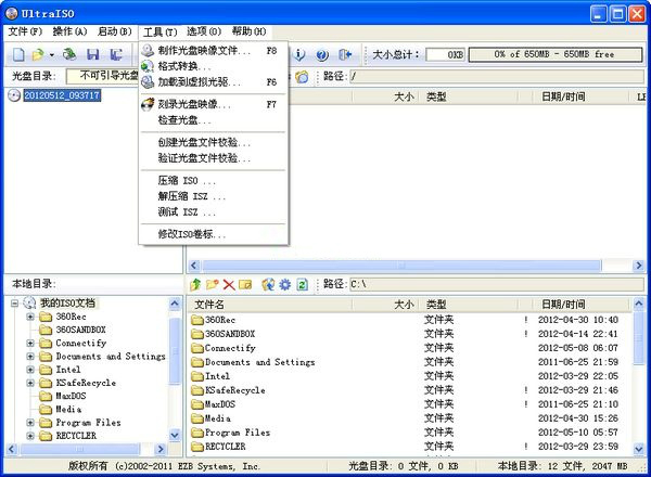

　　1.从CD-ROM制作光盘的映像文件。

　　2.将硬盘、光盘、网络磁盘文件制作成各种映像文件。

　　3.从ISO文件中提取文件或文件夹。

　　4.编辑各种映像文件(如Nero Burning ROM、Easy CD Creator、Clone CD 制作的光盘映像文件)。

　　5.UltraISO软碟通可以制作可启动ISO文件。

　　+ ) 新ISO文件处理内核，更稳定、高效

　　+)超强还原功能，可以准确还原被编辑文件，确保ISO文件不被损坏

　　+)可制作1.2M/1.44M/2.88M软盘仿真启动光盘

　　+)完整的帮助文件(CHM格式)

　　+)实现重新打开文件列表功能

　　+)支持Windows 2000下制作光盘映像文件

　　+)修正刻盘后有时出现目录不能打开错误。使用UltraISO，你可以随心所欲地制作/编辑光盘映像文件，配合光盘刻录软件烧录出自己所需要的光碟。

　　6.制作和编辑音乐CD文件

UltraISO软碟通软件特色

　　可以写入硬盘映像，从而可以制作启动U盘(新版本，如9.2、9.3)，制作的启动U盘启动类型有USB-HDD、USB-HDD+、USB-ZIP、USB-ZIP+，推荐选择USB-HDD。
　　● UltraISO软碟通可以直接编辑ISO文件
　　● 可以从光盘映像中直接提取文件和目录
　　● UltraISO软碟通支持对ISO文件任意添加/删除/新建目录/重命名
　　● 可以将硬盘上的文件制作成ISO文件
　　● 可以逐扇区复制光盘，制作包含引导信息的完整映像文件
　　● 可以处理光盘启动信息，你可以在 ISO 文件中直接添加/删除/获取启动信息
　　● UltraISO软碟通支持几乎所有已知的光盘映像文件格式(.ISO,..BIN,.CUE,.IMG,.CCD,.CIF,.NRG,.BWT,BWI,.CDI等)，并且将它们保存为标准的ISO格式文件
　　● 可直接设置光盘映像中文件的隐藏属性
　　● UltraISO软碟通支持ISO 9660 Level1/2/3和Joliet扩展
　　● 自动优化ISO文件存储结构，节省空间
　　● UltraISO软碟通支持shell文件类型关联，可在Windows资源管理器中通过双击或鼠标右键菜单打开ISO文件
　　● 双窗口操作，使用十分方便
　　● 配合选购插件，可实现N合1启动光盘制作、光盘映像文件管理，甚至软光驱，功能更强大

UltraISO软碟通安装步骤

1、首先在本站下载UltraISO软碟通软件包，下载完成后得到zip格式的压缩包，鼠标右键点击压缩包在弹出的菜单栏中选择解压到当前文件夹，得到exe安装文件，鼠标左键双击exe文件进入UltraISO软碟通安装向导界面，如下图所示，点击下一步继续安装。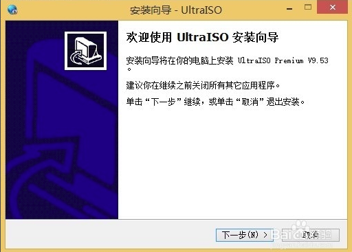

2、进入UltraISO软碟通许可协议界面，用户需要先阅读协议后点击界面左下角的我接受协议，才可以进行下一步，如果用户选择不接受协议，则无法进行安装。所以勾选“我接受”后，点击界面右下方的下一步选项。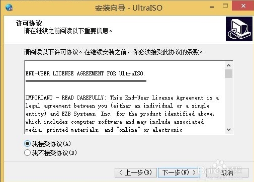

3、进入UltraISO软碟通安装位置选择界面，用户可以选择默认安装，直接点击下一步，软件会默认安装到系统C盘中，或者点击浏览选择自定义安装，选择合适的安装位置后再点击下一步。（小编建议用户选择自定义安装，将软件安装到其他盘中，C盘为系统盘，软件过多会导致电脑运行变慢。）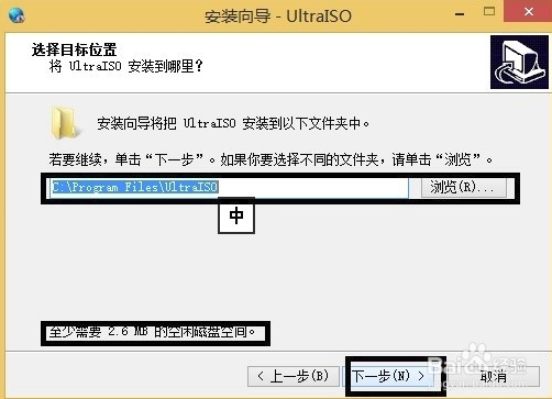

4、进入UltraISO软碟通开始菜单文件夹选择界面，用户可以选择默认的文件夹，或者点击浏览选择其他的文件夹，选择完成后点击界面下方的下一步。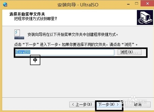

5、进入UltraISO软碟通附加任务选择界面，附加任务有在桌面创建图标、建立UltraISO 与.iso 文件关联和安装虚拟iOS驱动器三个选项，用户可以根据自己的需要选择勾选后在点击界面下方的下一步选项。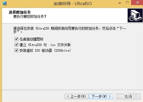

6、进入UltraISO软碟通准备安装界面，如下图所示，用户需要查看界面选框中的内容是否有问题，如果跟自己设置的都一样就可以点击界面下方的安装选项进行安装了。如果有问题可以点击上一步返回修改后再回到该界面点击安装。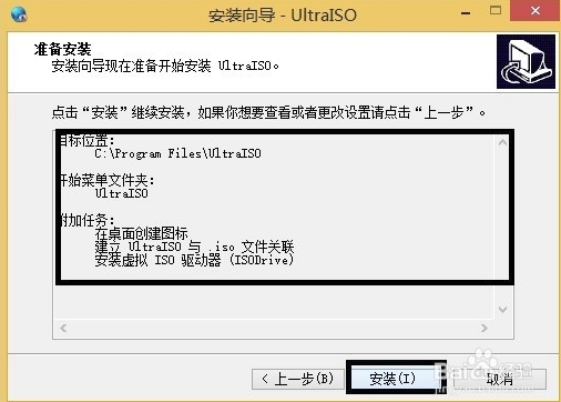

　7、UltraISO软碟通软件正在安装中，用户需要耐心等待安装进度条完成就可以完成安装了。小编亲测安装速度是很快的，用户只需等一下会就可以了。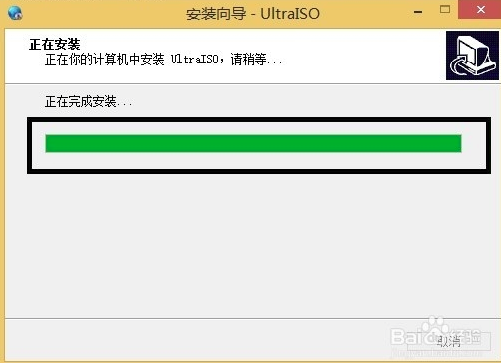

8、出现下图中的界面就表明UltraISO软碟通已经安装成功到用户的电脑上了，在界面还有查看README文件和运行UltraISO两个选项，用户可以取消勾选第一个，然后点击完成就可以关闭安装界面打开软件使用了。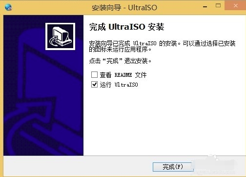

UltraISO软碟通制作u盘启动盘

　步骤一、首先在本站下载安装好UltraISO软碟通软件后，在桌面找到快捷方式鼠标左键双击运行软件进入主界面，接下来点击界面左上角的菜单【文件】，然后进入打开iOS文件界面，选择你的ISO路径，选定后点击界面下方的打开选项;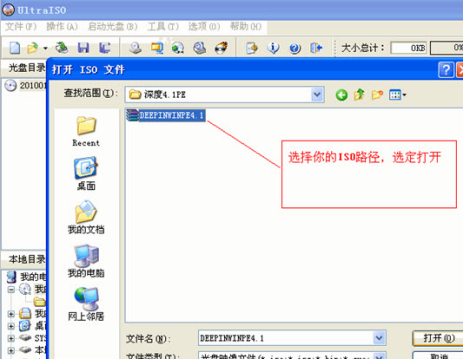

　步骤二、将ISO文件添加进来以后，用户再点击软件界面的启动光盘选项，然后在弹出的下拉选项中找到写入硬盘映像选项并点击，进入下一个界面。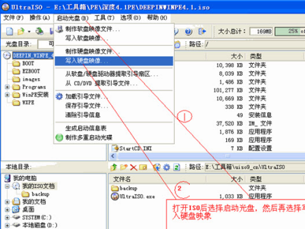

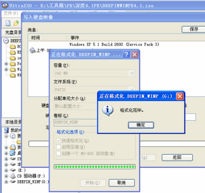
　步骤三、进入到写入硬盘映像界面，在界面下方选择硬盘驱动器(就是你的U盘盘符);选择完成后再点击界面下方的格式化，将U盘格式化一下。等待格式化完成后会提示用户格式化完毕，用户点击确定就可以了。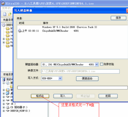


　步骤四、U盘格式化完成后，用户在写入硬盘映像界面还需要在选择写入方式，可选择：USB-HDD/USB-ZIP/USB-HDD+/USB-ZIP+ (小编选的是HDD+,选择完成后点击写入);然后等待程序提示刻录成功的信息后，就表示制作成功了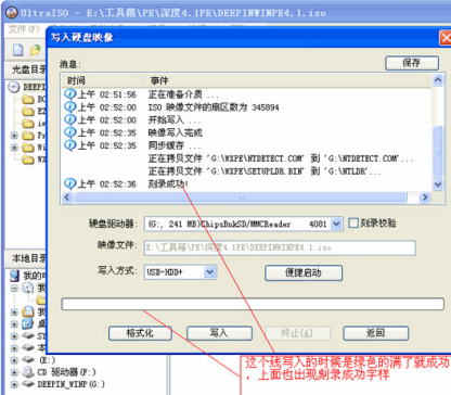

参考文献

UltraISO软碟通 9.6.5.3237 破解版含注册码

Windows下类似Linux下的命令

cmd下

1
2

c:\Users\Jack>for %x in (powershell.exe) do @echo %~$PATH:x
c:\Windows/System32\WindowPowerShell/v1.0\powershell.exe

powershell 下

``` PS C:\Users\Jack>Get-Command powershell.exe
CommandType Name Version Source

Application powershell.exe 10.0.17… C:\WINDOWS\System32\WindowsPowerShell...

Win10各种版本放出有一段时间了，而win10每次使用快捷键Win+E打开我的电脑（这台电脑）时，就变成了打开“快速访问”的文件夹，使用起来很不便，现在我们改回去以前windows的模式。

操作步骤

1.打开“这台电脑”

2.点击左上方菜单“查看”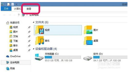

3.在下拉菜单右边打开“选项”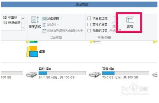

4.打开文件资源管理器以完成以下操作中选“这台电脑”，再点“应用”、“确定”即可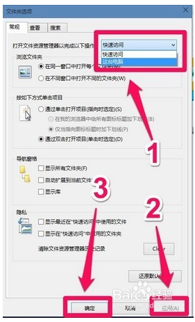

5.看看修改前使用WIN+E快捷键的样子：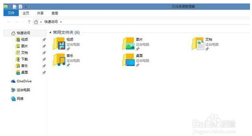

6.修改后的样子：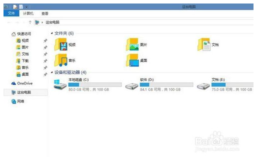

参考文献

• win10系统Win+E怎样改回打开我的电脑

tensorflow读取训练数据方法

预加载数据 Preloaded data

1
2
3
4
5
6
7
8
9
10
11
12
13

# coding: utf-8
import tensorflow as tf
 
# 设计Graph
x1 = tf.constant([2, 3, 4])
x2 = tf.constant([4, 0, 1])
y = tf.add(x1, x2)
 
with tf.Session() as sess:
  print sess.run(y)
 
# output:
# [6 3 5]

预加载数据方式是将训练数据直接内嵌到tf的图中，需要提前将数据加载到内存里，在数据量比较大，或者说在实际训练中，基本不可行。

声明占位符，运行时Feeding数据

1
2
3
4
5
6
7
8
9
10
11
12
13
14
15
16
17
18
19
20
21
22

# coding: utf-8
import tensorflow as tf
 
# 设计Graph
x1 = tf.placeholder(tf.int16)
x2 = tf.placeholder(tf.int16)
 
epoch_num = 0
 
# 用Python产生数据
data = [2, 3, 4]
label= [1, 0, 1]
 
with tf.Session() as sess:
  while epoch_num <len(data):
    print sess.run((x1,x2), feed_dict={x1: data[epoch_num], x2: label[epoch_num]})
    epoch_num+=1
    
# output:
# (array(2, dtype=int16), array(1, dtype=int16))
# (array(3, dtype=int16), array(0, dtype=int16))
# (array(4, dtype=int16), array(1, dtype=int16))

声明占位符是在训练过程中Feeding填充数据，可以选择把所有数据一次性加载到内存，每次取一个batch的数据出来训练，也可以选择把数据通过python建立一个生成器，每次加载一个batch的数据出来训练，加载方式比较灵活但是效率相对比较低。

从文件直接读取数据

从文件读取数据的方式是在Graph图中定义好文件读取的方式，在Session会话中启动（一个或多个）线程，把训练数据异步加载到内存（样本）队列中（先加载到文件名队列中，tf自动读取到内存队列中），通过队列管理器进行管理，执行效率较高，工作流程示意图：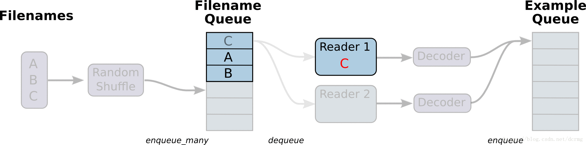

1
2
3
4
5
6
7
8
9
10
11
12
13
14
15
16
17
18
19
20
21
22
23
24
25
26
27
28
29
30
31
32
33
34
35
36
37
38
39
40
41
42
43
44
45
46
47
48
49
50
51
52
53
54
55
56
57
58
59
60
61
62
63
64
65
66
67
68
69
70
71
72
73
74
75
76

# -*- coding:utf-8 -*-
import tensorflow as tf
import numpy as np
 
# 样本个数
sample_num = 5
# 设置迭代次数
epoch_num = 2
# 设置一个批次中包含样本个数
batch_size = 3
# 计算每一轮epoch中含有的batch个数
batch_total = int(sample_num / batch_size) + 1
 
 
# 生成4个数据和标签
def generate_data(sample_num=sample_num):
    labels = np.asarray(range(0, sample_num))
    images = np.random.random([sample_num, 224, 224, 3])
    print('image size {},label size :{}'.format(images.shape, labels.shape))
    return images, labels
 
 
def get_batch_data(batch_size=batch_size):
    images, label = generate_data()
    # 数据类型转换为tf.float32
    images = tf.cast(images, tf.float32)
    label = tf.cast(label, tf.int32)
 
    # 从tensor列表中按顺序或随机抽取一个tensor准备放入文件名称队列
    input_queue = tf.train.slice_input_producer([images, label], num_epochs=epoch_num, shuffle=False)
 
    # 从文件名称队列中读取文件准备放入文件队列
    image_batch, label_batch = tf.train.batch(input_queue, batch_size=batch_size, num_threads=2, capacity=64,
                                              allow_smaller_final_batch=False)
    return image_batch, label_batch
 
 
image_batch, label_batch = get_batch_data(batch_size=batch_size)
 
with tf.Session() as sess:
    # 先执行初始化工作
    sess.run(tf.global_variables_initializer())
    sess.run(tf.local_variables_initializer())
 
    # 开启一个协调器
    coord = tf.train.Coordinator()
    # 使用start_queue_runners 启动队列填充
    threads = tf.train.start_queue_runners(sess, coord)
 
    try:
        while not coord.should_stop():
            print '************'
            # 获取每一个batch中batch_size个样本和标签
            image_batch_v, label_batch_v = sess.run([image_batch, label_batch])
            print(image_batch_v.shape, label_batch_v)
    except tf.errors.OutOfRangeError:  # 如果读取到文件队列末尾会抛出此异常
        print("done! now lets kill all the threads……")
    finally:
        # 协调器coord发出所有线程终止信号
        coord.request_stop()
        print('all threads are asked to stop!')
    coord.join(threads)  # 把开启的线程加入主线程，等待threads结束
    print('all threads are stopped!')  
    
# output:
# image size (5, 224, 224, 3),label size :(5,)
# ************
# ((3, 224, 224, 3), array([0, 1, 2], dtype=int32))
# ************
# ((3, 224, 224, 3), array([3, 0, 4], dtype=int32))
# ************
# ((3, 224, 224, 3), array([1, 2, 3], dtype=int32))
# ************
# done! now lets kill all the threads……
# all threads are asked to stop!
# all threads are stopped!

与从文件直接读取训练数据对应的还有一种方式是先把数据写入TFRecords二进制文件，再从队列中读取。

TFRecords方式相比直接读取训练文件，效率更高，特别是在训练文件比较多的情况下，缺点是需要额外编码处理TFRecords，不够直观。

Tensorflow 动态图机制（Eager Execution）下的Dataset数据读取

Tensorflow动态图机制支持图上的运算动态执行，更方便网络模型搭建和程序调试，不再需要通过sess.run()才能执行所定义的运算，调试时可以直接查看变量的值，做到了“所见即所得”，动态图运算应该是未来tensorflow发展的方向。
动图模式下就必须使用Dataset API来读取数据。
tensorflow 1.3 版本中，Dataset API是在contrib包的，1.4以后版本中，Dataset 放到了data中：

1
2

tf.contrib.data.Dataset  #1.3
tf.data.Dataset  # 1.4

Dataset 读取数据示例：

1
2
3
4
5
6
7
8
9
10
11
12
13
14
15
16
17
18
19
20

# -*- coding:utf-8 -*-
import tensorflow as tf
import numpy as np
 
dataset = tf.contrib.data.Dataset.from_tensor_slices(np.array([0,1,2,3,4,5]))
 
iterator = dataset.make_one_shot_iterator()
 
one_element = iterator.get_next()
 
with tf.Session() as sess:
  for i in range(5):
    print(sess.run(one_element))
 
# output:
# 0
# 1
# 2
# 3
# 4

Dataset 读取训练图片文件示例：

1
2
3
4
5
6
7
8
9
10
11
12
13
14
15
16
17
18
19

# 将图片文件名列表中的图片文件读入，缩放到指定的size大小
def _parse_function(filename, label, size=[128,128]):
  image_string = tf.read_file(filename)
  image_decoded = tf.image.decode_image(image_string)
  image_resized = tf.image.resize_images(image_decoded, size)
  return image_resized, label
 
# 图片文件名列表
filenames = tf.constant(["/var/data/image1.jpg", "/var/data/image2.jpg", ...])
 
# 图片文件标签
labels = tf.constant([0, 37, ...])
 
# 建立一个数据集，它的每一个元素是文件列表的一个切片
dataset = tf.data.Dataset.from_tensor_slices((filenames, labels))
# 对数据集中的图片文件resize
dataset = dataset.map(_parse_function)
# 对数据集中的图片文件组成一个一个batch，并对数据集扩展10次，相当于可以训练10轮
dataset = dataset.shuffle(buffersize=1000).batch(32).repeat(10)

参考文献

tensorflow读取训练数据方法

TensorFlow 数据读取方法总结

读取数据（Reading data）

TensorFlow输入数据的方法有四种：

• tf.data API：可以很容易的构建一个复杂的输入通道(pipeline)（首选数据输入方式）（Eager模式必须使用该API来构建输入通道）
• Feeding：使用Python代码提供数据，然后将数据feeding到计算图中。
• QueueRunner：基于队列的输入通道（在计算图计算前从队列中读取数据）
• Preloaded data：用一个constant常量将数据集加载到计算图中（主要用于小数据集）

文章目录

  读取数据（Reading data）

1. tf.data API
2. Feeding
3. QueueRunner
     3.1 Filenames, shuffling, and epoch limits
     3.2 File formats
       3.2.1 CSV file
       3.2.2 Fixed length records
       3.2.3 Standard TensorFlow format
     3.3 Preprocessing
     3.4 Batching
     3.5 Creating threads to prefetch using QueueRunner objects
     3.6 Filtering records or producing multiple examples per record
     3.7 Sparse input data
4. Preloaded data

5. Multiple input pipelines

6. tf.data API
   关于tf.data.Dataset的更详尽解释请看《programmer’s guide》。tf.data API能够从不同的输入或文件格式中读取、预处理数据，并且对数据应用一些变换（例如，batching、shuffling、mapping function over the dataset），tf.data API 是旧的 feeding、QueueRunner的升级。

参考文献
tensorflow之从文件中读取数据（适用场景：大规模数据集，亲测有效~）

TensorFlow 数据读取方法总结

GAN在图像生成应用综述（论文解读）

提示 “Unzip trin-images-idx3-ubyte.gz”，因此考虑安装gzip
search target1:Download Gzip.dll for Windows 10, 8.1, 8, 7, Vista and XP
Gzip.dll download. The Gzip.dll file is a dynamic link library for Windows 10, 8.1, 8, 7, Vista and XP. You can fix “The file Gzip.dll is missing.” and “Gzip.dll not found.” errors by downloading and installing this file from our site.

如何将gzip命令添加到Windows CMD？

Cygwin

Subprocess and Shell Commands in Python

Example Uses of the Linux gzip Command

windows 命令行使用 gzip

基础：tar 命令使用介绍

李云鹏个人博客

GNU Operating System

Cygwin

Cygwin安装配置

zip-gzip-bzip2_压缩文件

GZIP简介

GNU utilities for Win32

如何在命令行中提取gzip和tar文件

GNU Gzip

既香又贵的小飞跃：RTX2060替换了GTX1060

什么是JDK

  JDK是Java Development Kit的首字母缩写，意为Java开发工具包，是整个Java的核心。其不提供具体的开发软件，仅向程序员提供编写Java程序所必须的类库和Java语言规范。其包含以下三个版本：

• Java SE：Java标准环境
• Java EE：Java企业级环境
• Java ME：用于移动设备、嵌入式设备的Java环境

JDK包含哪些东西

JDK包含Java运行时环境(Java Runtime Environment,JRE)、Java工具集（如JConsole监控台）和Java的基础类库（如java.util包）。

在Windows10中怎么安装JDK

编者的电脑为Windows10 64位，因此以Windows10为例向大家展示JDK的安装过程。如有不懂的地方，请直接通过公众号向我提问哦！
第一步、下载JDK
一般开发者使用的是标准Java开发环境Java SE，因此我们打开以下网址：
https://www.oracle.com/technetwork/java/javase/overview/index.html, 所得界面如下：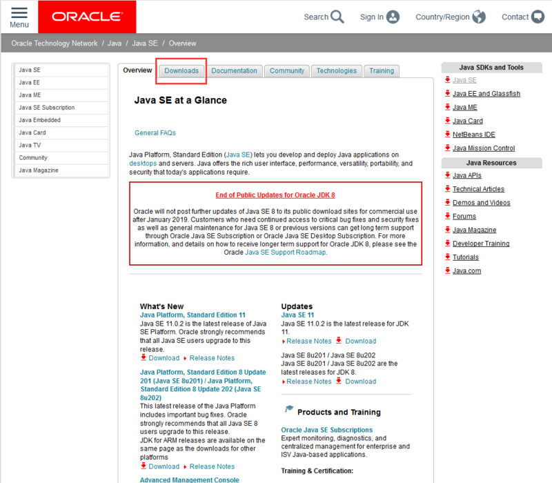

请注意途中红框的位置，我们要下载Java SE就得点这里。进去后是如下界面：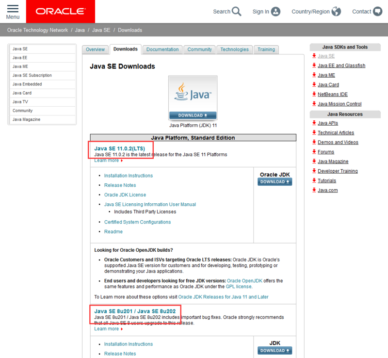

点进去后，我们发现有很多版本的JDK，这次我们安装使用人数比较多、比较稳定的JDK8，页面如下：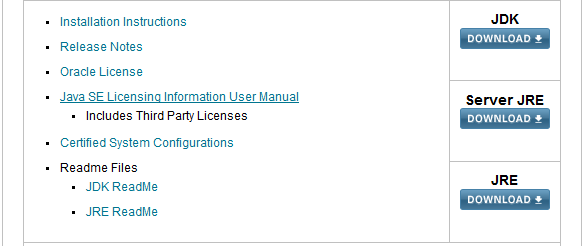

我们看到，其提供了三种下载的内容，JDK、Server JRE和JRE，这里我们是在本机开发使用，因此选择JDK，点击DOWNLOAD进入下载页：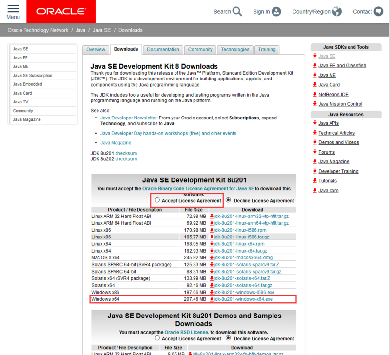

这个页面中提供了多个版本的JDK，这里我们选择第一个就好。先点击Accept License Agreement同意Oracle的开源协议，然后选择Windows x64位进行下载（记得一定要先同意协议哦）

第二步、开始安装
下载完成后，双击进行安装，界面如下：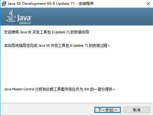

点下一步，在这一步中要选择安装路径，这个路径一定要记住，待会儿有大用处：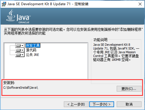

然后点下一步进行安装，这个过程可能会持续几分钟，之后会出现如下这个界面：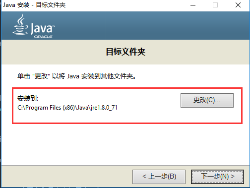

这里需要选择的是JRE的安装路径，这个路径也请记住了，点下一步就开始安装了：


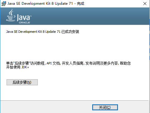
安装完毕了，直接点关闭即可。

第三步、设置环境变量
 &emspp;一般JDK安装完成后，都会进行环境变量设置，目的是让系统能够找到java和javac命令。不过现在程序的傻瓜式安装，一般情况下会自动给你配置好，但是为了安全起见，我们还是要检查下：
请按以下步骤点击：鼠标选中我的电脑 -> 右键 -> 属性，出现如下界面：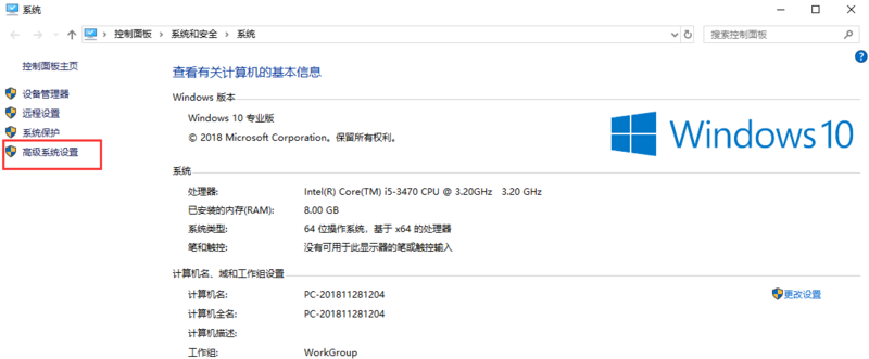

点击高级系统设置 -> 环境变量，出现如下界面：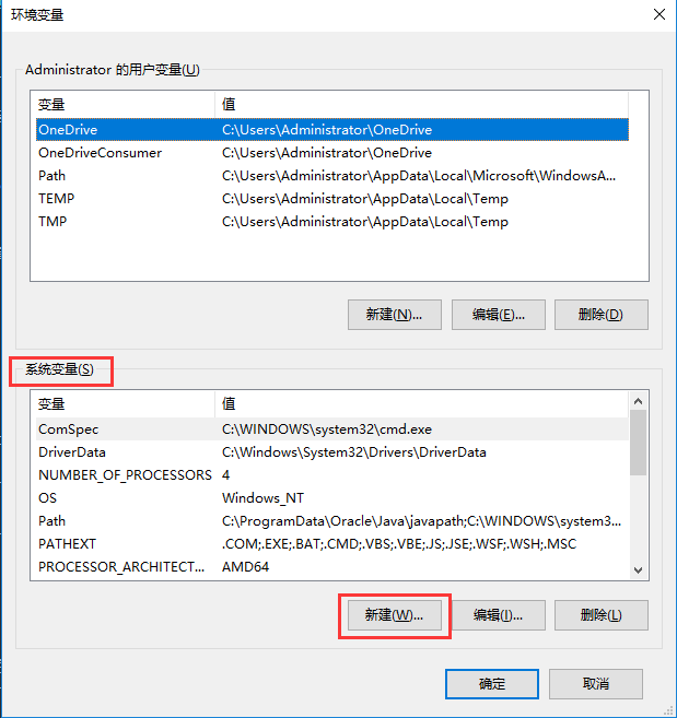

我们在下方系统变量栏目中，点击新建，新建类目如下：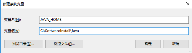

• 变量名：JAVA_HOME
• 变量值：你的JDK的安装路径，记住，是JDK，不是JRE，比如我的JDK路径是：C:\SoftwareInstall\Java\jdk-12.0.1

设置完成后，点击确定；然后我们再点新建，设置另一个环境变量：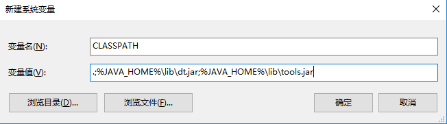

• 变量名：CLASSPATH
• 变量值：.;%JAVA_HOME%libdt.jar;%JAVA_HOME%libtools.jar,一定要记住前面的.;哦！

  最后，我们还需要在一个名为Path的变量中加入Java的环境信息。首先找到Path变量（大小写请忽略，系统可能不同），然后点击编辑，紧接着前面的环境变量后面加上%JAVA_HOME%\bin;%JAVA_HOME%\jre\bin;，在你添加的环境和原环境之间，记得用;隔开哦！

到这里，环境变量就设置完成啦！

第四步、验证安装
现在请按下Windows+R，就是那个四叶窗图标+R，然后输入cmd并回车，在命令行中键入java -version，如果出现了如下界面，显示了Java的版本信息，就是配置成功啦！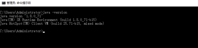

恭喜你，迈出了成功的第一步！

总结

  本文讲述了在Windows10环境中安装JDK的过程。在其他版本的Windows中也大同小异。如果读者遇到其他问题，欢迎在公众号中向我提问，或者在我的博客中留言！下一节的番外篇2中，将会向大家讲述Java中比较重要的几个关键字及编码规范。
  于20190521，安装jdk-12.0.1的过程中，发现安装过程中并没有提示要安装jre，故此次安装仅仅安装了jdk文件。

JDK下载网站

https://www.oracle.com/technetwork/java/javase/downloads/index.html

参考文献

• 番外篇1：在Windows环境下安装JDK
• jdk版本的选择（推荐1.8）
• Java - 安装jdk并设置环境变量

Tqdm 是一个快速，可扩展的Python进度条，可以在 Python 长循环中添加一个进度提示信息，用户只需要封装任意的迭代器 tqdm(iterator)。
基本用法：

1
2
3

from tqdm import tqdm
for i in tqdm(range(10000)):
     sleep(0.01)

当然除了tqdm，还有trange,使用方式完全相同

1
2
3
4
5
6
7
8
9

for i in trange(100):
        sleep(0.1)
```        

只要传入list都可以：
``` python 
pbar = tqdm(["a", "b", "c", "d"])
for char in pbar:
    pbar.set_description("Processing %s" % char)

也可以手动控制更新

1
2
3

with tqdm(total=100) as pbar:
    for i in range(10):
        pbar.update(10)

也可以这样：

1
2
3
4

pbar = tqdm(total=100)
for i in range(10):
    pbar.update(10)
pbar.close()

参考文献

• 【CSDN】(2017年01月31日)python的Tqdm模块

Github站点：

• 各种GAN的介绍-GAN note.md
• 嵌入式AI 双周简报 (2018-01-31)

博文站点：

• (Keras)动手实现会写数字的神经网络—半监督学习和生成式对抗网络介绍
  Semi-Supervised Learning and GANs

• (code)Semi-supervised learning with GANs

(KDD2018)Semi-Supervised Generative Adversarial Network for Gene Expression Inference

(developer-mayuan)Semi-Supervised GAN
(GAN系列)developer-mayuan

Semi-Supervised Haptic Material Recognition using GANs

生成对抗网络 半监督分类

http://pwp.gatech.edu/hrl/mr-gan/

前言

买了新的笔电并成功配置了Win10上面的tensorflow的GPU版

毕竟稍微大一点的神经网路CPU跑起来实在慢的要人命!

纪录了一些流程希望帮助也在安装的朋友省一点时间

可以赶快开始利用新买的显卡来工作或做程式学习

配置流程

首先下载并安装Anaconda+Python3.7的版本

https://www.anaconda.com/distribution/

下载后直接参考tensorflow官网的说明

不要相信来路不明的教学啦QQ乖乖照着TensorFlow-gpu官网做才是最准的!!!
我们需要做的事情有:

1
2
3

1. 确认GPU驱动有更新
2. CUDA@Tookit 10.0安装
3. cuDNN SDK 7.5(forCUDA 10.0)安装

官方网址：https://www.tensorflow.org/install/gpu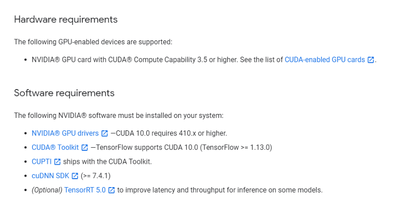

配置方案，可以参考下图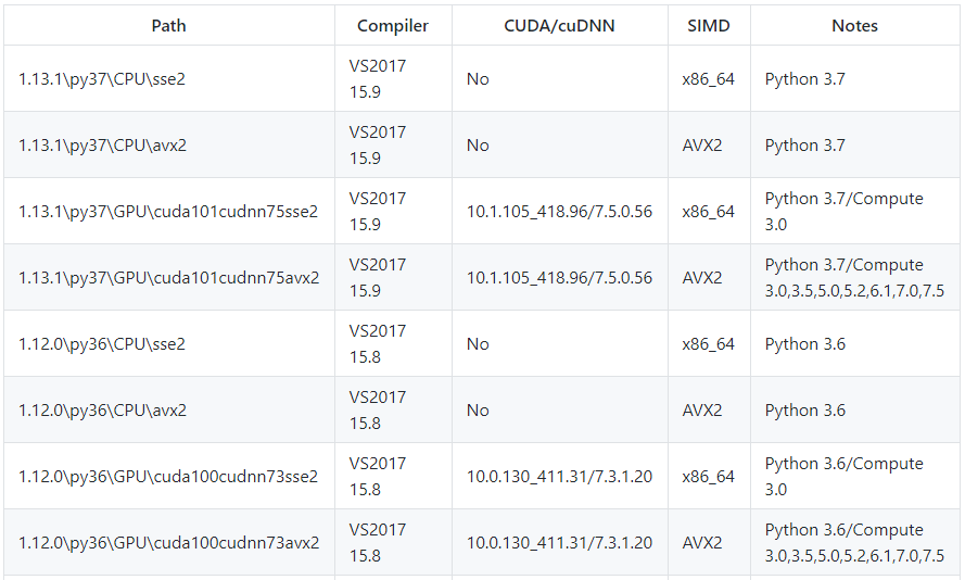

照着上面的标示安装必要程序
1.显卡驱动因为刚买来还满新的进Geforce Experience更新一下不用重载
根据显卡驱动，选择对应的CUDA版本号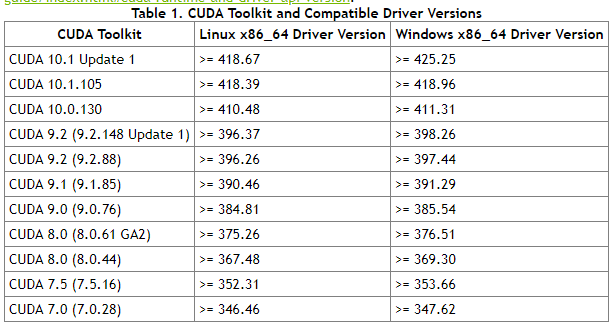

查看本机的显卡驱动版本号，方法如下：
  WIN+R，输入CMD，然后输入”nvidia-smi”，即可显示对应的显卡驱动版本号，有些还会显示对应的支持CUDA的版本号，本机验证CUDA支持10.0。

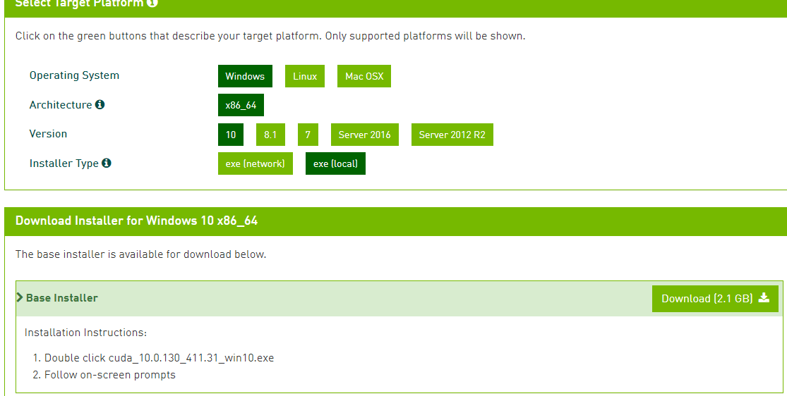
2.下载CUDA 10.0 + CUDNN7.5 for 10.0 (版本记得要一样喔不然会错误)

• 1.下载CUDA 10.0, CUDA Toolkit Archive
  

如想了解是否正确安装可以

1

nvcc - V

如果成功应该是如下图所示：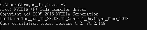

• 2.下载CUDNN
   &emspp;直接去NVDIA官网去下载就好啦~大家想要下载，还需要注册NVDIA账户，很麻烦，不过下载好像可以直接微信登录了，我没试过，大家就直接微信登录就好啦,下面附上链接：下载链接
  这里面有好几个for CUDA10.0的，大家一定要注意，因为关系到我们后面tensorflow的版本，这里出错了，后面就会报错！！！ 这里我们选择cuDNN v7.5的版本
  到这里下载完成！完成后咱们开始解压，然后将相应的包，放到cuda相应包底下。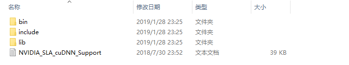
  
  咱们只需要拿出这些文件夹里面文件放到想要cuda文件夹即可，我的cuda文件夹地址为：
  C:\Program Files\NVIDIA GPU Computing Toolkit\CUDA\v10.0
  供大家参考。

1. TensorFlow-GPU下载和安装
   
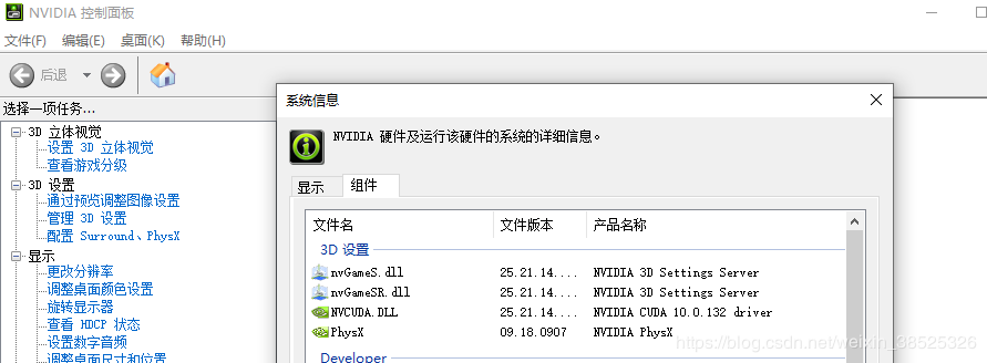
   我们可以通过进入英伟达控制面板，点击帮助，选择系统信息，再点组件，看到我们的RTX 2060显卡是支持CUDA10。
   前面我让大家下载了CUDA9.2,没坑大家哦，CUDA9.2也是支持RTX 2060的。tensoeflow官方现在无论哪个版本都不支持，所以我们还是去求助Github！！！

安装

1
2

// An highlighted block
pip install tensorflow_gpu

测试

1
2
3
4
5

// An highlighted block
import tensorflow as tf
hello = tf.constant('Hello, TensorFlow!')
sess = tf.Session()
print(sess.run(hello))

结果

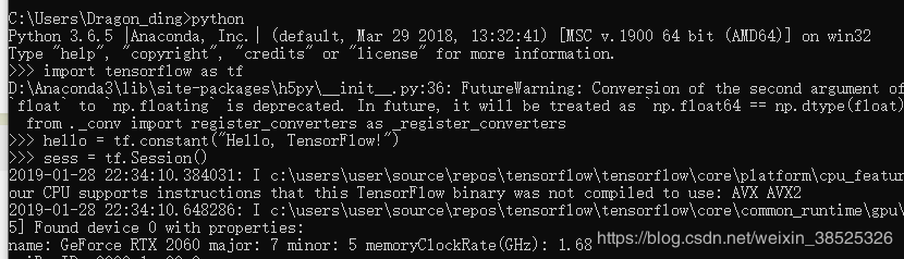
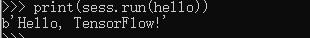
已经能够识别出RTX2060显卡了，并成功输出！到这里也算完成了，大家安装遇到的坑也欢迎来交流！

常用网址

1. CUDA Toolkit Archive
2. cuDNN Archive
3. Tensorflow prebuilt binary for Windows
4. TensorFlow-gpu官网

参考文献

• 【CSDN】(2019年01月29日 11:48:14)RTX2060+win10+Tensorflow GPU+CUDA 9.2+CUDNN7.2+python 3.65
• 【Blog】(2019年3月24日)WIN10+CUDA10 +CUDNN7.5+ TENSORFLOW-GPU1.13.1 + python3.7 运行NVIDIA STYLEGAN 的安装过程和踩坑实录
• 【Medium】(2019年4月27日)Win10 + RTX 2060 + tensorflow GPU

ImportError: No module named cv2 报错处理

内容

• 在安装opevncv时会出现 ImportError: No module named cv2 的错误，找不到cv2的包。
• 这时候安装扩展包即可：

  1	pip install opencv-python

参考地址

ImportError: No module named cv2 报错处理

前沿

配置环境，研究了一整天，踩了很多坑，在网上找了很多资料，发现基本上都没非常明确的教程，所以今天想分享一下配置tensorflow GPU版本的经验，希望能让各位朋友少走些弯路。（PS：一切的前提，你需要有一张Nvidia显卡。我的显卡是 GT940MX）

Tensorflow有两个版本：GPU和CPU版本，CPU的很好安装；GPU 版本需要 CUDA 和 cuDNN 的支持，如果你是独显+集显，那么推荐你用GPU版本的，因为GPU对矩阵运算有很好的支持，会加速程序执行！并且CUDA是Nvidia下属的程序，所以你的GPU最好是Nvidia的，AMD的显卡没有CUDA加速！满足以上条件之后，你需要查看一下你的英伟达GPU是否支持CUDA，以下是Geforce支持的目录：

你也可以点击查看你的GPU是否支持CUDA

满足以上条件之后，你就可以安装Tensorflow了！

第一步：安装Anaconda

1.下载和安装
下载地址：https://www.anaconda.com/download/

我系统是64位，所以下载 64-Bit Graphical Installer (631 MB)，之后就是进行安装了。

和安装其他软件没有什么区别，需要注意的是这一步，不要勾选“Add Anaconda to my PATH enviroment variable”，我们后面会手动加入。

接下来就是等待了，安装结束后需要测试是否能正常使用，打开CMD输入“conda”命令，发现提示“’conda’ is not recognized as an internal or external command, operable program or batch file.”

这是由于我们没有配置环境变量的原因。

2.配置Anaconda环境变量
我们点击左下角搜索栏搜索“环境变量”

点击环境变量

选择“Path”，点击“编辑”

将以下三个路径加入，注意这里要换成你自己的安装路径。

• C:\Users\t-yaoguo\AppData\Local\Continuum\anaconda3
• C:\Users\t-yaoguo\AppData\Local\Continuum\anaconda3\Scripts
• C:\Users\t-yaoguo\AppData\Local\Continuum\anaconda3\Library\bin
  
  然后点击“确定”保存，这回再测试一下，再cmd中输入“conda -V”，能正常显示版本号，证明已经配置好了。
  

第二步：安装TensorFlow-GPU

打开tensorflow官网：https://www.tensorflow.org/install/install_windows#installing_with_anaconda

跟着操作步骤走就可以了。

1.创建conda环境
通过调用下列命令，创建一个名为“tensorflow”的conda环境：

1

conda create -n tensorflow pip python=3.5

等待相应包的安装，如果国内网络太慢的话，可以为conda设置清华源，这样速度能快一点，具体配置过程，网上查一下吧，此处不再讲述。如果看到这样的提示，就证明conda环境创建成功。

2.激活环境
通过以下命令激活conda环境：

1

activate tensorflow

这样就进入了刚创建的“tensorflow”环境。

3.安装tensorflow-gpu
安装GPU版本的tensorflow需要输入以下命令：

1

pip install --ignore-installed --upgrade tensorflow-gpu

如果只需要安装CPU版本的tensorflow则输入以下命令：

1

pip install --ignore-installed --upgrade tensorflow

这样就安装成功了。

注意：务必注意一点，在安装完tensroflow后，由于我们是新创建的conda环境，该环境中基本上是空的，有很多包和IDE并没有安装进来，例如“Ipython”，“spyder”此时如果我们在该环境下打开spyder/Ipyton/jupyter notebook等，会发现其实IDE使用的kernel并不是新建立的这个环境的kernel，而是“base”这个环境的，而“base”环境中我们并没有安装tensorflow，所以一定无法import。这也就是为什么有很多人在安装好tensorflow后仍然在IDE里无法正常使用的原因了。

通过以下命令安装Anaconda基础包

1

conda install anaconda

这回，我们测试一下是否能import tensorflow

程序报错，这是由于我们虽然安装好了tensorflow-gpu，但是还需要安装CUDA Toolkit 和 cuDNN。

第三步：安装CUDA Toolkit + cuDNN

1.查看需要安装的CUDA+cuDNN版本
注意，tensorflow是在持续更新的，具体安装的CUDA和cuDNN版本需要去官网查看，要与最新版本的tensorflow匹配。

点击查看最新tensorflow支持的CUDA版本：
https://www.tensorflow.org/install/install_windows#requirements_to_run_tensorflow_with_gpu_support

现在（PS：此博客书写日期 2018年7月5日）最新版tensorflow支持的是 CUDA® Toolkit 9.0 + cuDNN v7.0，一定注意，安装的版本一定一定要正确，不要看NVIDIA官网推出CUDA® Toolkit 9.2了就感觉最新版的更好，而安装最新版，这样很可能会导致tensorflow无法正常使用，所以一定要跟着tensorflow 官网的提示来。

2.下载CUDA + cuDNN
在这个网址查找CUDA已发布版本：https://developer.nvidia.com/cuda-toolkit-archive

进入下载界面

下载好CUDA Toolkit 9.0 后，我们开始下载cuDnn 7.0，需要注意的是，下载cuDNN需要在nvidia上注册账号，使用邮箱注册就可以，免费的。登陆账号后才能下载。

cuDNN历史版本在该网址下载：https://developer.nvidia.com/rdp/cudnn-archive


这样，我们就下载好了 CUDA Toolkit 9.0 和 cuDnn 7.0，下面我们开始安装。

3.安装 CUDA Toolkit 9.0 和 cuDnn 7.0
至关重要的一步：卸载显卡驱动
由于CUDA Toolkit需要在指定版本显卡驱动环境下才能正常使用的，所以如果我们已经安装了nvidia显卡驱动（很显然，大部分人都安装了），再安装CUDA Toolkit时，会因二者版本不兼容而导致CUDA无法正常使用，这也就是很多人安装失败的原因。而CUDA Toolkit安装包中自带与之匹配的显卡驱动，所以务必要删除电脑先前的显卡驱动。
安装


此处选择“自定义（高级）”

勾选所有

一路通过即可。

接下来，解压“cudnn-9.0-windows10-x64-v7.zip”，将一下三个文件夹，拷贝到CUDA安装的根目录下。

这样CUDA Toolkit 9.0 和 cuDnn 7.0就已经安装了，下面要进行环境变量的配置。

配置环境变量
将下面四个路径加入到环境变量中，注意要换成自己的安装路径。

1
2
3
4
5
6
7

C:\Program Files\NVIDIA GPU Computing Toolkit\CUDA\v9.0

C:\Program Files\NVIDIA GPU Computing Toolkit\CUDA\v9.0\bin

C:\Program Files\NVIDIA GPU Computing Toolkit\CUDA\v9.0\lib\x64

C:\Program Files\NVIDIA GPU Computing Toolkit\CUDA\v9.0\libnvvp

到此，全部的安装步骤都已经完成，这回我们测试一下。

第四步：测试

1.查看是否使用GPU

1
2

import tensorflow as tf
tf.test.gpu_device_name()

2.查看在使用哪个GPU

1
2

from tensorflow.python.client import device_lib
device_lib.list_local_devices()

好了大功告成！

参考文献

Win10 Anaconda下TensorFlow-GPU环境搭建详细教程（包含CUDA+cuDNN安装过程）

有朋友反馈说安装不了Package Control
研究了一下，之前Host的列表把ST3的全都屏蔽了
仔细想了想有点智障，只用屏蔽license server就行
已更新，新的host就没问题了。
感谢@eui620的提醒

我没在win下开发的习惯…
抱歉没发现WinHex不能保存超过200K的文件
用这个在线编辑器吧，啥平台都行。
https://hexed.it

1. 下载软件

官网: 点我下载
网盘地址见底部

2. 安装软件

这个我就不多BB了。
安装完请勿打开SublimeText3。
（若已打开关了就是）

破解”>3. 破解

3207版本基本杜绝了共享license key的方法
所以我们要修改验证license时的trigger
因官方采用revoke illegal licenses的方式，即使当时显示激活成功，联网验证时便会凉凉。

所以我们还要采用hosts屏蔽法复制以下地址直接粘贴到相应系统的hosts文件内

1
2
3
4

127.0.0.1 license.sublimehq.com
127.0.0.1 www.sublimetext.com
50.116.34.243 sublime.wbond.net
50.116.34.243 packagecontrol.io

3.1 修改trigger

3.1.1 Win

• 利用WinHex(网盘会有)或其他HexEditor打开软件根目录下的sublime_text.exe
• 搜索16进制 97 94 0D 00
• 改为 00 00 00 00
• 保存

3.1.2 Mac

• 拷出/Applications/Sublime Text.app/Contents/MacOS/Sublime Text

• 其实就是 应用程序 文件夹下找到SublimeText应用，然后右键->显示包内容，然后打开/Contents/MacOS/ 然后找到 Sublime Text 这个文件 拷出来

• 利用0xED(网盘会有)或者其他HexEditor打开它

• 搜索16进制 97 94 0D 00
• 改为 00 00 00 00
• 如果实在不会修改网盘里有修改好的现成的
• 保存
• 打开终端，切换到当前目录
• 然后键入chmod 755 Sublime Text
• 替换掉/Applications/Sublime Text.app/Contents/MacOS/Sublime Text
• 完事儿

3.1.3 Linux

基本同Mac操作

• 找个16进制编辑器打开软件根目录下的Sublime Text
• 搜索16进制 97 94 0D 00
• 改为 00 00 00 00
• 保存
• 打开终端，切换到当前目录
• 然后键入chmod 755 Sublime Text
• 完事儿

3.2 修改host

3.2.1 Win

Windows的hosts文件在：
系统盘:/windows/system32/drivers/etc/hosts

1
2

Tips: Win下的权限获取可能有点复杂，不如先拷到桌面，编辑完替换回去。
在最后一行插入

1
2
3
4

127.0.0.1 license.sublimehq.com
127.0.0.1 www.sublimetext.com
50.116.34.243 sublime.wbond.net
50.116.34.243 packagecontrol.io

3.2.2 Mac

1. 打开Terminal(终端)
2. 输入 sudo nano /Private/etc/hosts 回车
3. 输入密码后回车

4. 在最后一行插入

   1 2 3 4

   127.0.0.1 license.sublimehq.com 127.0.0.1 www.sublimetext.com 50.116.34.243 sublime.wbond.net 50.116.34.243 packagecontrol.io

5. 按下Control + X，输入Y确定修改，确认保存路径后敲击回车

3.2.3 Linux

同Mac

4. 激活

打开Sublime Text 3
选择Help -> Enter License
输入

1
2
3
4
5
6
7
8
9
10
11
12
13

----- BEGIN LICENSE -----
TwitterInc
200 User License
EA7E-890007
1D77F72E 390CDD93 4DCBA022 FAF60790
61AA12C0 A37081C5 D0316412 4584D136
94D7F7D4 95BC8C1C 527DA828 560BB037
D1EDDD8C AE7B379F 50C9D69D B35179EF
2FE898C4 8E4277A8 555CE714 E1FB0E43
D5D52613 C3D12E98 BC49967F 7652EED2
9D2D2E61 67610860 6D338B72 5CF95C69
E36B85CC 84991F19 7575D828 470A92AB
------ END LICENSE ------

选择Use license

5.大功告成

6.中文化

不知道该不该写，好多人觉得哇人家破解版带个汉化猴赛雷
其实在Package Control就有 Rexdf 翻译的插件

• 按下command + shift + p(win或linux为 ctrl + shift + p) 输入 install 选择 Install Package Control
  
• 等待提示安装完成
• 完成后按下command + shift + p(win或linux为 ctrl + shift + p) 输入 install 选择 Package Control: Install Package
  
• 输入 localization 选择 ChineseLocalizitions
  
• 等待提示安装完成
• 大功告成，如需切换语言选择help -> Languages
  

7.附件

附件什么附件？？
我这破等级还想发附件？？？
卑微，蚂蚁花卑，葡萄美酒夜光卑…..
百度网盘 密码:lksz

问答

（发表于 2019-4-16 08:08，by hjner）

我测试，说注册码不对…..XP 下测试的。

第二次重装，同样出现 ：
plugin_host has exited unexpectedly,plugin functionality won’t be available until Sublime Text has been restarted

不关闭程序，先设置好HOST文件，屏蔽服务器，然后，直接 输入注册码，反而通过！
之前重启程序在输入注册码，则无效。

谢谢，成功！

安装中文时候，出现
installing package control,出现提示，访问
https://packagecontrol.io/installation

手动安装，

但是网站进不去…只有以后再试试了。

(发表于 2019-5-7 16:36 by 花了19元)

127.0.0.1 license.sublimehq.com
127.0.0.1 www.sublimetext.com
50.116.34.243 sublime.wbond.net
50.116.34.243 packagecontrol.io

激活成功，但是这样修改hosts，插件安装不了。

解决办法(https://www.jianshu.com/p/23b823d6e786)：
点击 Preferences > Package Settings > Package Control > Settings - User
添加配置
“channels”: [“https://raw.githubusercontent.com/HBLong/channel_v3_daily/master/channe

理论介绍

  我研究这个是因为发现右键菜单在安装了一下软件后，越来越臃肿，有用的没用的菜单项都被塞进去了，于是自己动手给菜单瘦个身。

  这里首先警告一句：下面操作全部涉及到修改注册表，看见不认识，不确定的注册表项，别手欠看见空项或者自以为无用的注册表项，就瞎乱删。最好是有一定操作注册表的基础在跟着本文操作，至少要知道怎么备份和恢复注册表。手欠的孩子都请自己准备好恢复或重装系统，本文的经过作者本人亲自实践无误，但不保证文中描述完全正确或适用于所有版本的win10操作系统。如果在按照本文说明操作时，发生了系统崩溃，死机，或其他任何可修复/不可修复的系统问题，你可以顺着网线来打我啊，然而我也救不了你。

  首先，所有的右键菜单项，几乎都可以在注册表中设置。按 Win + R 打开“ 运行…”窗口，输入 regedit ，按回车键打开。注意：注册表编辑器是需要管理员权限的。

打开注册表，根项展开有5个子项，如上图所示。右键菜单的项目都包含在第一子项 HKEY_CALSS_ROOT 中。展开该项，第一个子项一般是 * ，这个统配符表示一切后缀的文件都通用。也就是说，这个子项中的一切右键菜单项，没有特别说明，会出现每一个文件的右键菜单中。

展开这一子项，在其内部，所有的右键菜单分为两部分存储（我也懒得去搞清楚这两块区域有什么不同），见下图：

用红线圈起来的两个注册表键，就是放置了右键菜单的地方，看看有哪些是自己安装的软件带来的，看名字挑着没用的就能删除了。这里特别提醒一句，看见键名称是一串序列号的，请仔细核对后，确认不是系统项再删除。用这种长串数字当名字的键，如果里面空空如也，那很有可能是系统项。

然后是文件夹，文件夹分为两类菜单，一类是鼠标指向一个文件夹图标时，点击右键出来的菜单；第二类菜单时鼠标在已经打开的文件夹窗口的空白处，点击右键弹出的菜单。如下图所示，第一类菜单的注册表项直接在 Directory 下，shell和shellex\ContextMenuHandlers 里面；第二类菜单则在子项 Background 里面。

哦，对了，还有比较特殊的桌面菜单。在桌面空白处点击右键，弹出的菜单在 DesktopBackground 项里面：

是的，细心的人应该已经发现了，这里的菜单项不全。是的，不全，然而我也不知道其他的在哪里，懒得找……

然后还有一些，比如：
驱动器（就是C盘、光驱，之类那些，带着卷标的），在 Drive 项里面；
文件夹还有一些在 Folder 项里面；
字体文件的在 fontfile 项里面；
等等…… 英文好的同学可以自行发挥了。

上面讲的是如何找到一些项，然后就能删除里面多余的菜单项。下面将一些添加项的方法：

以python文件为例（*.py），python如见有两个大分支：2.x系列和3.x系列。那么有时候我们的机器上会同时安装这两个python的运行环境，这时候想要快速的用python解释器打开某个*.py文件，要么就是命令行，要么就是频繁更改打开方式，要么就是来回挪动环境变量的前后顺序……好吧，我不废话了，下面开始动手添加右键菜单。

首先，还是找到包含python脚本文件的右键菜单项的注册表键，完整的路径是 Computer\HKEY_CLASSES_ROOT\pysFile ，如下图。这里可以看到，有3个子项。一眼可以看到右键菜单的藏身之处：

一般安装python时，附带的菜单项倒在 Shell 子键里面，展开，把一串什么 runwithidle 之类的统统干掉，然后我们来加入自己的项。
右键点击 Shell ，然后选择 新建 ，然后选择 键：

简单点的话，不做附加设置，这个键的名字就会是右键菜单项的显示名字，如下图所示：

之后，如果更改这个键的默认值，就会更改菜单的显示名字：

只有一个键，是不能让这个菜单项真正生效的，这时如果点击这个菜单项，就会收到系统发出的错误警告。下面来添加点击这个菜单项所触发的命令：
在新建的键里面（图里面的 MieHaHa键），再新建一个键，命名为 command，一般大小写都行，但是我还是建议全小写吧。然后更改这个键的默认值，双击(Default)（中文操作系统这里应该是默认），会弹出修改框，把值修改为你的python.exe所在完整路径+参数就可以了，比如我的python36安装在D:\Environment\Python36\python.exe, 那么我这里就要输入 "D:\Environment\Python36\python.exe" "%1" %*。这里简单解释一下，这里的值，就相当与是命令行里敲的命令。因为是点击文件弹出的菜单， %1 就是被点击的py文件的完整路径。

有了这个菜单项，就能使用这一项直接用python运行脚本文件了。然而，这也太简陋了，看好多程序都用dll文件，把自己的菜单项折叠成了一个子菜单组，简洁又方便。在WIN10里，其实不用dll，只用注册表，也能自己制作一个折叠的子菜单组，比如上图（图8）的 Run With 项就是我自己写的一个菜单组。下图直接上键的树：

除了最内层两个 command 和 最外层的 runwith 其余的键都没有值。 runwith 里需要新建两个 字符串的值：一个命名为 MUIVerb，值为 &Run With，也就是这个菜单组的名称，注意要以 & 开头，这个字符不会被显示；第二个值，命名为Subcommands，没有值。如下图：

将 Sublime Text 添加到系统右键菜单栏的方法

Sublime Text 是一个代码编辑器（Sublime Text 2是收费软件，但可以无限期试用），也是HTML和散文先进的文本编辑器。Sublime Text是由程序员Jon Skinner于2008年1月份所开发出来，它最初被设计为一个具有丰富扩展功能的Vim。
Sublime Text具有漂亮的用户界面和强大的功能，例如代码缩略图，Python的插件，代码段等。还可自定义键绑定，菜单和工具栏。Sublime Text 的主要功能包括：拼写检查，书签，完整的 Python API ， Goto 功能，即时项目切换，多选择，多窗口等等。Sublime Text 是一个跨平台的编辑器，同时支持Windows、Linux、Mac OS X等操作系统。（摘自百度百科）

咳咳，废话少说，切入正题：
这么好的编译器在打开需要编译的文件时却存在一个非常让人头疼的问题：不能右键菜单选择使用 Sublime text 打开！！！

下面为大家介绍一种通过修改系统注册表的方法将 Sublime text 添加到右键菜单中：

1. 首先使用 Win + R 打开运行，输入 regedit 按下回车键进入注册表；
   
   运行后进入注册表界面：
   

2. 依次展开 HKEY_CLASSES_ROOT -> * -> shell，右键 shell 新建一个项并命名为：Open With Sublime Text 如图：
   

3. 双击选中新建项 Open With Sublime Text ，在右边展示栏空白处右键新建字符串值，数值名称填 lcon ，数值数据填 E:\Sublime Text3\sublime_text.exe,0 （注意：路径请改成你安装Sublime Text 的路径喔）
   
   

4. 右键新建的 Open With Sublime Text 新建一个项，命名为 Command （注意：请必须命名为 Command 喔），并双击选中 Command ，在右边的展示栏中将默认项的数值数据修改为：E:\Sublime Text 3\sublime_text.exe “%1” （注意：1、将我的路径改成你安装 Sublime Text 的路径，2、”必须要写喔）
   
   
   进行到这里，右键菜单的 Open With Sublime Text 选项就实现啦！！！

sublime text 添加到鼠标右键功能

Sublime Text是一款具有代码高亮、语法提示、自动完成且反应快速的编辑器软件，不仅具有华丽的界面，还支持插件扩展机制，用她来写代码，绝对是一种享受。如何把sublime text添加到鼠标右键，以方便我们使用呢？

方法与步骤

1.在Windows系统中，下载并安装sublime text3 软件，（可以到sublime text3 的官方网站下载），如下图，可以按不同的系统选择下载安装包。

2.下载完成后，双击安装包文件进行安装，安装比较简单，按照提示点击“下一步”，最后完成安装，如下图所示。

3.sublime text 添加到鼠标右键功能：把以下内容复制并保存到文件，重命名为：sublime_addright.reg，然后双击就可以了。
（注意：需要把下面代码中的Sublime的安装目录（标粗部分），替换成自已实际的Sublime安装目录）

1
2
3
4
5
6
7
8
9
10
11
12
13
14
15
16
17
18
19
20
21

Windows Registry Editor Version 5.00

[HKEY_CLASSES_ROOT\*\shell\SublimeText3]

@="用 SublimeText3 打开"

"Icon"="C:\\Program Files\\Sublime Text 3\\sublime_text.exe,0"

[HKEY_CLASSES_ROOT\*\shell\SublimeText3\command]

@="C:\\Program Files\\Sublime Text 3\\sublime_text.exe %1"

[HKEY_CLASSES_ROOT\Directory\shell\SublimeText3]

@="用 SublimeText3 打开"

"Icon"="C:\\Program Files\\Sublime Text 3\\sublime_text.exe,0"

[HKEY_CLASSES_ROOT\Directory\shell\SublimeText3\command]

@="C:\\Program Files\\Sublime Text 3\\sublime_text.exe %1"

其中，@=”用 SublimeText3 打开” 引号中的内容为出现在鼠标右键菜单中的文字内容。
4.双击文件sublime_addright.reg 完成后，鼠标选中要编辑的文件，点击鼠标右键，弹出菜单，其中就会出现刚才添加的“用 SublimeText3 打开”选项，如下图所示。

将Sublime Text 添加到鼠标右键的方法

步骤:

1. win+R 打开运行，并输入regedit。
2. 在左侧依次打开HKEY_CLASSES_ROOT*\shell

3. 在shell下新建“Sublime Text”项，在右侧窗口的“默认”键值栏内输入“用Sublime Text打开”。项的名称和键值可以任意，最好是和程序关联起来。其中键值将显示在右键菜单中。

4. 在“用Sublime Text打开”下再新建Command项，在右侧窗口的“默认”键值栏内输入Sublime Text程序所在的路径,在路径后添加 %1。%1表示要打开的文件参数。

5. 关闭注册表窗口，立即生效。（如图）
   

注意事项：

    1. 第四步时的Command无法自定义。必须输入Command才可以。
    2. 输入程序路径时注意为以下格式：例. d:\sub\sub.exe %1

  万事不要太依赖别人，自己动手才能丰衣足食。这个鼠标右键也可以使用第三方程序来调用添加，而且这个改注册表不止方便，还可以举一反三，做的更多。
  附上下载链接这个中文不会乱码: 链接：https://pan.baidu.com/s/1jH9KD8a 密码：p6du

参考文献

• Win10如何自定义右键菜单-修改注册表（图文
• 将 Sublime Text 添加到系统右键菜单栏的方法
• sublime text 添加到鼠标右键功能
• 将Sublime Text 添加到鼠标右键的方法
• win10右键菜单修改，任意位置打开cmd命令行程序

  In this post I will cover a partial re-implementation of a recent paper on manifold regularization (Lecouat et al., 2018) for semi-supervised learning with Generative Adversarial Networks (Goodfellow et al., 2014). I will attempt to re-implement their main contribution, rather than getting all the hyperparameter details just right. Also, for the sake of demonstration, time constraints and simplicity, I will consider the MNIST dataset rather than the CIFAR10 or SVHN datasets as done in the paper. Ultimately, this post aims at bridging the gap between the theory and implementation for GANs in the semi-supervised learning setting. The code that comes with this post can be found here.

Generative Adversarial Networks

  Let’s quickly go over Generative Adversarial Networks (GAN). In terms of the current pace within the AI/ML community, they have been around for a while (just about 4 years), so you might already be familiar with them. The ‘vanilla’ GAN procedure is to train a generator to generate images that are realistic and capable of fooling a discriminator. The generator generates the images by means of a deep neural network that takes in a noise vector z.
  The discriminator (which is a deep neural network as well) is fed with the generated images, but also with some real data. Its job is to say whether each image is either real (coming from the dataset) or fake (coming from the generator), which in terms of implementation comes down to binary classification. The image below summarizes the vanilla GAN setup.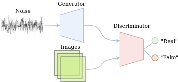

Semi-supervised learning

  Semi-supervised learning problems concern a mix of labeled and unlabeled data. Leveraging the information in both the labeled and unlabeled data to eventually improve the performance on unseen labeled data is an interesting and more challenging problem than merely doing supervised learning on a large labeled dataset. In this case we might be limited to having only about 200 samples per class. So what should we do when only a small portion of the data is labeled?
  Note that adversarial training of vanilla GANs doesn’t require labeled data. At the same time, the deep neural network of the discriminator is able to learn powerful and robust abstractions of images by gradually becoming better at discriminating fake from real. Whatever it’s learning about unlabeled images will presumably also yield useful feature descriptors of labeled images. So how do we use the discriminator for both labeled and unlabeled data? Well, the discriminator is not necessarily limited to just telling fake from real. We could decide to train it to also classify the real data.
  A GAN with a classifying discriminator would be able to exploit both the unlabeled as well as the labeled data. The unlabeled data will be used to merely tell fake from real. The labeled data would be used to optimize the classification performance. In practice, this just means that the discriminator has a softmax output distribution for which we minimize the cross-entropy. Indeed, part of the training procedure is just doing supervised learning. The other part is about adversarial training. The image below summarizes the semi-supervised learning setup with a GAN.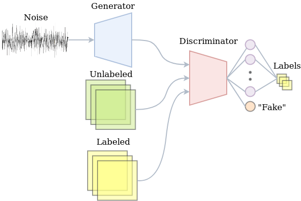

The implementation

  Let’s just head over to the implementation, since that might be the best way of understanding what’s happening. The snippet below prepares the data. It doesn’t really contain anything sophisticated. Basically, we take 400 samples per class and concatenate the resulting arrays as being our actual supervised subset. The unlabeled dataset consists of all train data (it also includes the labeled data, since we might as well use it anyway). As is customary for training GANs now, the output of the generator uses a hyperbolic tangent function, meaning its output is between -1 and +1. Therefore, we rescale the data to be in that range as well. Then, we create TensorFlow iterators so that we can efficiently go through the data later without having to struggle with feed dicts later on.

1
2
3
4
5
6
7
8
9
10
11
12
13
14
15
16
17
18
19
20
21
22
23
24
25
26
27
28
29
30
31
32
33
34
35
36
37
38
39
40
41
42
43
44
45
46
47
48
49
50
51
52
53
54
55
56
57
58
59
60
61
62

def prepare_input_pipeline(flags_obj):
    (train_x, train_y), (test_x, test_y) = tf.keras.datasets.mnist.load_data(
        "/home/jos/datasets/mnist/mnist.npz")

    def reshape_and_scale(x, img_shape=(-1, 28, 28, 1)):
        return x.reshape(img_shape).astype(np.float32) / 255. * 2.0 - 1.0

    # Reshape data and rescale to [-1, 1]
    train_x = reshape_and_scale(train_x)
    test_x = reshape_and_scale(test_x)

    # Shuffle train data
    train_x_unlabeled, train_y_unlabeled = shuffle(train_x, train_y)

    # Select subset as supervised
    train_x_labeled, train_y_labeled = [], []
    for i in range(flags_obj.num_classes):
        train_x_labeled.append(
            train_x_unlabeled[train_y_unlabeled == i][:flags_obj.num_labeled_examples])
        train_y_labeled.append(
            train_y_unlabeled[train_y_unlabeled == i][:flags_obj.num_labeled_examples])
    train_x_labeled = np.concatenate(train_x_labeled)
    train_y_labeled = np.concatenate(train_y_labeled)

    with tf.name_scope("InputPipeline"):

        def train_pipeline(data, shuffle_buffer_size):
            return tf.data.Dataset.from_tensor_slices(data)\
                .cache()\
                .shuffle(buffer_size=shuffle_buffer_size)\
                .batch(flags_obj.batch_size)\
                .repeat()\
                .make_one_shot_iterator()

        # Setup pipeline for labeled data
        train_ds_lab = train_pipeline(
            (train_x_labeled, train_y_labeled.astype(np.int64)),
            flags_obj.num_labeled_examples * flags_obj.num_classes)
        images_lab, labels_lab = train_ds_lab.get_next()

        # Setup pipeline for unlabeled data
        train_ds_unl = train_pipeline(
            (train_x_unlabeled, train_y_unlabeled.astype(np.int64)), len(train_x_labeled))
        images_unl, labels_unl = train_ds_unl.get_next()

        # Setup another pipeline that also uses the unlabeled data, so that we use a different
        # batch for computing the discriminator loss and the generator loss
        train_x_unlabeled, train_y_unlabeled = shuffle(train_x_unlabeled, train_y_unlabeled)
        train_ds_unl2 = train_pipeline(
            (train_x_unlabeled, train_y_unlabeled.astype(np.int64)), len(train_x_labeled))
        images_unl2, labels_unl2 = train_ds_unl2.get_next()

        # Setup pipeline for test data
        test_ds = tf.data.Dataset.from_tensor_slices((test_x, test_y.astype(np.int64)))\
            .cache()\
            .batch(flags_obj.batch_size)\
            .repeat()\
            .make_one_shot_iterator()
        images_test, labels_test = test_ds.get_next()

    return (images_lab, labels_lab), (images_unl, labels_unl), (images_unl2, labels_unl2), \
           (images_test, labels_test)

  Next up is to define the discriminator network. I have deviated quite a bit from the architecture in the paper. I’m going to play safe here and just use Keras layers to construct the model. Actually, this enables us to very conveniently reuse all weights for different input tensors, which will prove to be useful later on. In short, the discriminator’s architecture uses 3 convolutions with 5x5 kernels and strides of 2x2, 2x2 and 1x1 respectively. Each convolution is followed by a leaky ReLU activation and a dropout layer with a dropout rate of 0.3. The flattened output of this stack of convolutions will be used as the feature layer.
  The feature layer can be used for a feature matching loss (rather than a sigmoid cross-entropy loss as in vanilla GANs), which has proven to yield a more reliable training process. The part of the network up to this feature layer is defined in _define_tail in the snippet below. The _define_head method defines the rest of the network. The ‘head’ of the network introduces only one additional fully connected layer with 10 outputs, that correspond to the logits of the class labels. Other than that, there are some methods to make the interface of a Discriminator instance behave similar to that of a tf.keras.models.Sequential instance.

1
2
3
4
5
6
7
8
9
10
11
12
13
14
15
16
17
18
19
20
21
22
23
24
25
26
27
28
29
30
31
32
33
34
35
36
37
38
39
40
41
42
43
44
45
46
47
48

class Discriminator:

    def __init__(self):
        """The discriminator network. Split up in a 'tail' and 'head' network, so that we can
        easily get the """
        self.tail = self._define_tail()
        self.head = self._define_head()

    def _define_tail(self, name="Discriminator"):
        """Defines the network until the intermediate layer that can be used for feature-matching
        loss."""
        feature_model = models.Sequential(name=name)

        def conv2d_dropout(filters, strides, index=0):
            # Adds a convolution followed by a Dropout layer
            suffix = str(index)
            feature_model.add(layers.Conv2D(
                filters=filters, strides=strides, name="Conv{}".format(suffix), padding='same',
                kernel_size=5, activation=tf.nn.leaky_relu))
            feature_model.add(layers.Dropout(name="Dropout{}".format(suffix), rate=0.3))

        # Three blocks of convs and dropouts. They all have 5x5 kernels, leaky ReLU and 0.3
        # dropout rate.
        conv2d_dropout(filters=32, strides=2, index=0)
        conv2d_dropout(filters=64, strides=2, index=1)
        conv2d_dropout(filters=64, strides=1, index=2)

        # Flatten it and build logits layer
        feature_model.add(layers.Flatten(name="Flatten"))
        return feature_model

    def _define_head(self):
        # Defines the remaining layers after the 'tail'
        head_model = models.Sequential(name="DiscriminatorHead")
        head_model.add(layers.Dense(units=10, activation=None, name="Logits"))
        return head_model

    @property
    def trainable_variables(self):
        # Return both tail's parameters a well as those of the head
        return self.tail.trainable_variables + self.head.trainable_variables

    def __call__(self, x, *args, **kwargs):
        # By adding this, the code below can treat a Discriminator instance as a
        # tf.keras.models.Sequential instance
        features = self.tail(x, *args, **kwargs)
        return self.head(features, *args, **kwargs), features

  The generator’s architecture also uses 5x5 kernels. Many implementations of DCGAN-like architectures use transposed convolutions (sometimes wrongfully referred to as ‘deconvolutions’). I have decided to give the upsampling-convolution alternative a try. This should alleviate the issue of the checkerboard pattern that sometimes appears in generated images. Other than that, there are ReLU nonlinearities, and a first layer to go from the 100-dimensional noise to a (rather awkwardly shaped) 7x7x64 spatial representation.

1
2
3
4
5
6
7
8
9
10
11
12
13
14
15
16
17
18
19
20
21

def define_generator():
    model = models.Sequential(name="Generator")

    def conv2d_block(filters, upsample=True, activation=tf.nn.relu, index=0):
        if upsample:
            model.add(layers.UpSampling2D(name="UpSampling" + str(index), size=(2, 2)))
        model.add(layers.Conv2D(
            filters=filters, kernel_size=5, padding='same', name="Conv2D" + str(index),
            activation=activation))

    # From flat noise to spatial
    model.add(layers.Dense(7 * 7 * 64, activation=tf.nn.relu, name="NoiseToSpatial"))
    model.add(layers.Reshape((7, 7, 64)))

    # Four blocks of convolutions, 2 that upsample and convolve, and 2 more that
    # just convolve
    conv2d_block(filters=128, upsample=True, index=0)
    conv2d_block(filters=64, upsample=True, index=1)
    conv2d_block(filters=64, upsample=False, index=2)
    conv2d_block(filters=1, upsample=False, activation=tf.nn.tanh, index=3)
    return model

  I have tried to make this model work with what TensorFlow’s Keras layers have to offer so that the code would be easy to digest (and to implement of course). This also means that I have deviated from the architectures in the paper (e.g. I’m not using weight normalization). Because of this experimental approach, I have also experienced just how sensitive the training setup is to small variations in network architectures and parameters. There are plenty of neat GAN ‘hacks’ listed here which I definitely found insightful.

Putting it together

  Let’s do the forward computations now so that we see how all of the above comes together. This consists of setting up the input pipeline, noise vector, generator and discriminator. The snippet below does all of this. Note that when define_generator returns the Sequential instance, we can just use it as a functor to obtain the output of it for the noise tensor given by z.
  The discriminator will do a lot more. It will take (i) the ‘fake’ images coming from the generator, (ii) a batch of unlabeled images and finally (iii) a batch of labeled images (both with and without dropout to also report the train accuracy). We can just repetitively call the Discriminator instance to build the graph for each of those outputs. Keras will make sure that the variables are reused in all cases. To turn off dropout for the labeled training data, we have to pass training=False explicitly.

1
2
3
4
5
6
7
8
9
10
11
12
13
14
15
16
17
18
19
20
21
22
23

(images_lab, labels_lab), (images_unl, labels_unl), (images_unl2, labels_unl2), \
            (images_test, labels_test) = prepare_input_pipeline(flags_obj)

with tf.name_scope("BatchSize"):
    batch_size_tensor = tf.shape(images_lab)[0]

# Get the noise vectors
z, z_perturbed = define_noise(batch_size_tensor, flags_obj)

# Generate images from noise vector
with tf.name_scope("Generator"):
    g_model = define_generator()
    images_fake = g_model(z)
    images_fake_perturbed = g_model(z_perturbed)

# Discriminate between real and fake, and try to classify the labeled data
with tf.name_scope("Discriminator") as discriminator_scope:
    d_model = Discriminator()
    logits_fake, features_fake          = d_model(images_fake, training=True)
    logits_fake_perturbed, _            = d_model(images_fake_perturbed, training=True)
    logits_real_unl, features_real_unl  = d_model(images_unl, training=True)
    logits_real_lab, features_real_lab  = d_model(images_lab, training=True)
    logits_train, _                     = d_model(images_lab, training=False)

The discriminator’s loss

  Recall that the discriminator will be doing more than just separating fake from real. It also classifies the labeled data. For this, we define a supervised loss which takes the softmax output. In terms of implementation, this means that we feed the unnormalized logits to tf.nn.sparse_cross_entropy_with_logits.
  Defining the loss for the unsupervised part is where things get a little bit more involved. Because the softmax distribution is overparameterized, we can fix the unnormalized logit at 0 for an image to be fake (i.e. coming from the generator). If we do so, the probability of it being real just turns into:

  where Z(x) is the sum of the unnormalized probabilities. Note that we currently only have the logits. Ultimately, we want to use the log-probability of the fake class to define our loss function. This can now be achieved by computing the whole expression in log-space:

  Where the lower case l with subscripts denote the individual logits. Divisions become subtractions and sums can be computed by the logsumexp function. Finally, we have used the definition of the softplus function:

  In general, if you have the log-representation of a probability, it is numerically safer to keep things in log-space for as long as you can, since we are able to represent much smaller numbers in that case.
  We’re not there yet. Generative adversarial training asks us to ascend the gradient of:

  So whenever we call tf.train.AdamOptimizer.minimize we should descent:

  The first term on the right-hand side of the equation can be written:

  The second term of the right-hand side can be written as:

  So that finally, we arrive at the following loss:

1
2
3
4
5
6
7
8
9
10
11
12
13
14
15

# Set the discriminator losses
with tf.name_scope("DiscriminatorLoss"):
    # Supervised loss, just cross-entropy. This normalizes p(y|x) where 1 <= y <= K
    loss_supervised = tf.reduce_mean(tf.nn.sparse_softmax_cross_entropy_with_logits(
        labels=labels_lab, logits=logits_real_lab))

    # Sum of unnormalized log probabilities
    logits_sum_real = tf.reduce_logsumexp(logits_real_unl, axis=1)
    logits_sum_fake = tf.reduce_logsumexp(logits_fake, axis=1)
    loss_unsupervised = 0.5 * (
        tf.negative(tf.reduce_mean(logits_sum_real)) +
        tf.reduce_mean(tf.nn.softplus(logits_sum_real)) +
        tf.reduce_mean(tf.nn.softplus(logits_sum_fake)))
    loss_d = loss_supervised + loss_unsupervised

Optimizing the discriminator

  Let’s setup the operations for actually updating the parameters of the discriminator. We will just reside to the Adam optimizer. While tweaking the parameters before I wrote this post, I figured I might slow down the discriminator by setting its learning rate at 0.1 times that of the generator. After that my results got much better, so I decided to leave it there for now. Notice also that we can very easily select the subset of variables corresponding to the discriminator by exploiting the encapsulation offered by Keras.

1
2
3
4
5

# Configure discriminator training ops
with tf.name_scope("Train") as train_scope:
    optimizer = tf.train.AdamOptimizer(flags_obj.lr * 0.1)
    optimize_d = optimizer.minimize(loss_d, var_list=d_model.trainable_variables)
    train_accuracy_op = accuracy(logits_train, labels_lab)

Adding some control flow to the graph

  After we have the new weights for the discriminator, we want the generator’s update to be aware of the updated weights. TensorFlow will not guarantee that the updated weights will actually be used even if we were to redeclare the forward computation after defining the minimization operations for the discriminator. We can still force this by using tf.control_dependencies. Any operation defined in the scope of this context manager will depend on the evaluation of the ones that are passed to context manager at instantiation. In other words, our generator’s update that we define later on will be guaranteed to compute the gradients using the updated weights of the discriminator.

1
2
3
4
5

with tf.name_scope(discriminator_scope):
    with tf.control_dependencies([optimize_d]):
        # Build a second time, so that new variables are used
        logits_fake, features_fake = d_model(images_fake, training=True)
        logits_real_unl, features_real_unl = d_model(images_unl2, training=True)

The generator’s loss and updates

  In this implementation, the generator tries to minimize the L2 distance of the average features of the generated images vs. the average features of the real images. This feature-matching loss (Salimans et al., 2016) has proven to be more stable for training GANs than directly trying to optimize the discriminator’s probability for observing real data. It is straightforward to implement. While we’re at it, let’s also define the update operations for the generator. Notice that the learning rate of this optimizer is 10 times that of the discriminator.

1
2
3
4
5
6
7
8
9
10
11

# Set the generator loss and the actual train op
with tf.name_scope("GeneratorLoss"):
    feature_mean_real = tf.reduce_mean(features_real_unl, axis=0)
    feature_mean_fake = tf.reduce_mean(features_fake, axis=0)
    # L1 distance of features is the loss for the generator
    loss_g = tf.reduce_mean(tf.abs(feature_mean_real - feature_mean_fake))

with tf.name_scope(train_scope):
    optimizer = tf.train.AdamOptimizer(flags_obj.lr, beta1=0.5)
    train_op = optimizer.minimize(loss_g, var_list=g_model.trainable_variables)

Adding manifold regularization

  Lecouat et. al (2018) propose to add manifold regularization to the feature-matching GAN training procedure of Salimans et al. (2016). The regularization forces the discriminator to yield similar logits (unnormalized log probabilities) for nearby points in the latent space in which z resides. It can be implemented by generating a second perturbed version of z and computing the generator’s and discriminator’s outputs once more with this slightly altered vector.

  This means that the noise generation code looks as follows:

1
2
3
4
5
6
7
8

def define_noise(batch_size_tensor, flags_obj):
    # Setup noise vector
    with tf.name_scope("LatentNoiseVector"):
        z = tfd.Normal(loc=0.0, scale=flags_obj.stddev).sample(
            sample_shape=(batch_size_tensor, flags_obj.z_dim_size))
        z_perturbed = z + tfd.Normal(loc=0.0, scale=flags_obj.stddev).sample(
            sample_shape=(batch_size_tensor, flags_obj.z_dim_size)) * 1e-5
    return z, z_perturbed

  The discriminator’s loss will be updated as follows (note the 3 extra lines at the bottom):

1
2
3
4
5
6
7
8
9
10
11
12
13
14
15
16
17

# Set the discriminator losses
with tf.name_scope("DiscriminatorLoss"):
    # Supervised loss, just cross-entropy. This normalizes p(y|x) where 1 <= y <= K
    loss_supervised = tf.reduce_mean(tf.nn.sparse_softmax_cross_entropy_with_logits(
        labels=labels_lab, logits=logits_real_lab))

    # Sum of unnormalized log probabilities
    logits_sum_real = tf.reduce_logsumexp(logits_real_unl, axis=1)
    logits_sum_fake = tf.reduce_logsumexp(logits_fake, axis=1)
    loss_unsupervised = 0.5 * (
        tf.negative(tf.reduce_mean(logits_sum_real)) +
        tf.reduce_mean(tf.nn.softplus(logits_sum_real)) +
        tf.reduce_mean(tf.nn.softplus(logits_sum_fake)))
    loss_d = loss_supervised + loss_unsupervised
    if flags_obj.man_reg:
        loss_d += 1e-3 * tf.nn.l2_loss(logits_fake - logits_fake_perturbed) \
            / tf.to_float(batch_size_tensor)

Classification performance

  So how does it really perform? I have provided a few plots below. There are many things I might try to squeeze out additional performance (for instance, just training for longer, using a learning rate schedule, implementing weight normalization), but the main purpose of writing this post was to get to know a relatively simple yet powerful semi-supervised learning approach. After 100 epochs of training, the mean test accuracy approaches 98.9 percent.
  The full script can be found here. Thanks for reading!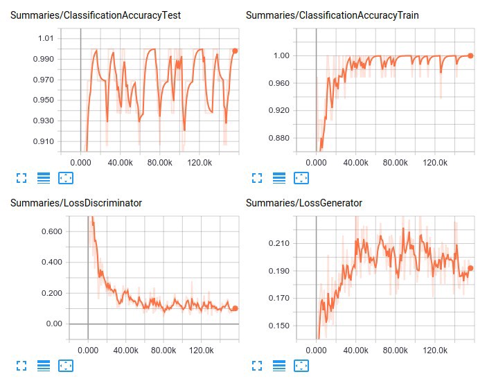

Reference

• Semi-supervised learning with GANs

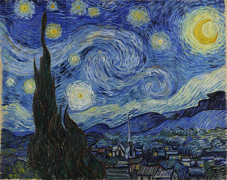
  Vincent Van Gogh painted this beautiful art: ‘The Starry Night’ in 1889 and today my GAN model (I like to call it GAN Gogh :P) painted some MNIST digits with only 20% labeled data!! How could it achieve this remarkable feat? … Let’s find out

Introduction

What is semi-supervised learning?
  Most deep learning classifiers require a large amount of labeled samples to generalize well, but getting such data is an expensive and difficult process. To deal with this limitation Semi-supervised learning is presented, which is a class of techniques that make use of a morsel of labeled data along with a large amount of unlabeled data.Many machine-learning researchers have found that unlabeled data, when used in conjunction with a small amount of labeled data can produce considerable improvement in learning accuracy. GANs have shown a lot of potential in semi-supervised learning where the classifier can obtain a good performance with very few labeled data.

Background on GANs
  GANs are members of deep generative models. They are particularly interesting because they don’t explicitly represent a probability distribution over the space where the data lies. Instead, they provide some way of interacting less directly with this probability distribution by drawing samples from it.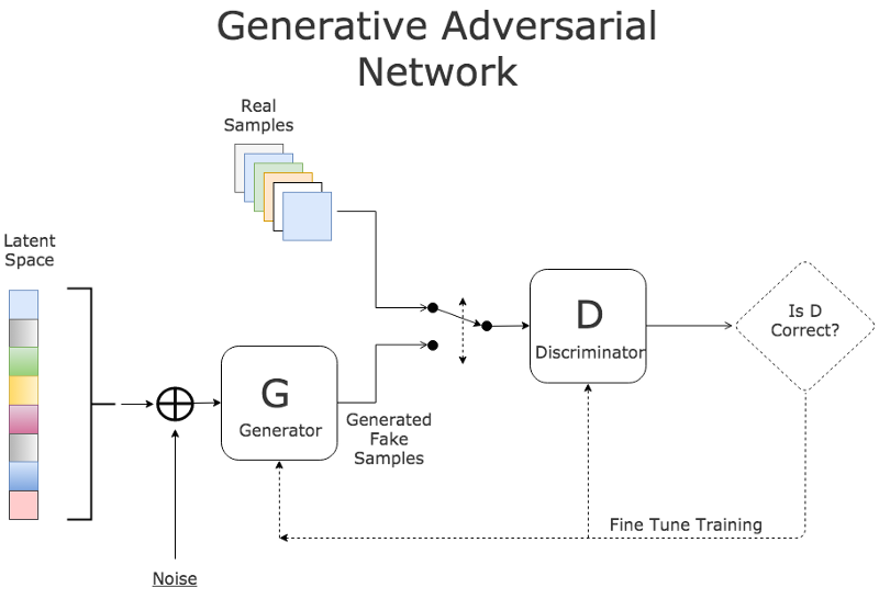

The basic idea of GAN is to set up a game between two players:

• A generator G: Takes random noise z as input and outputs an image x. Its parameters are tuned to get a high score from the discriminator on fake images that it generates.
• A discriminator D: Takes an image x as input and outputs a score which reflects its confidence that it is a real image. Its parameters are tuned to have a high score when it is fed by a real image, and a low score when a fake image is fed from the generator.

  I suggest you to go through this and this for more details on their working and optimisation objectives. Now, let us turn the wheels a little and talk about one of the most prominent applications of GANs, semi-supervised learning.

Intuition

  The vanilla architecture of discriminator has only one output neuron for classifying the R/F probabilities. We train both the networks simultaneously and discard the discriminator after the training as it was used only for improving the generator.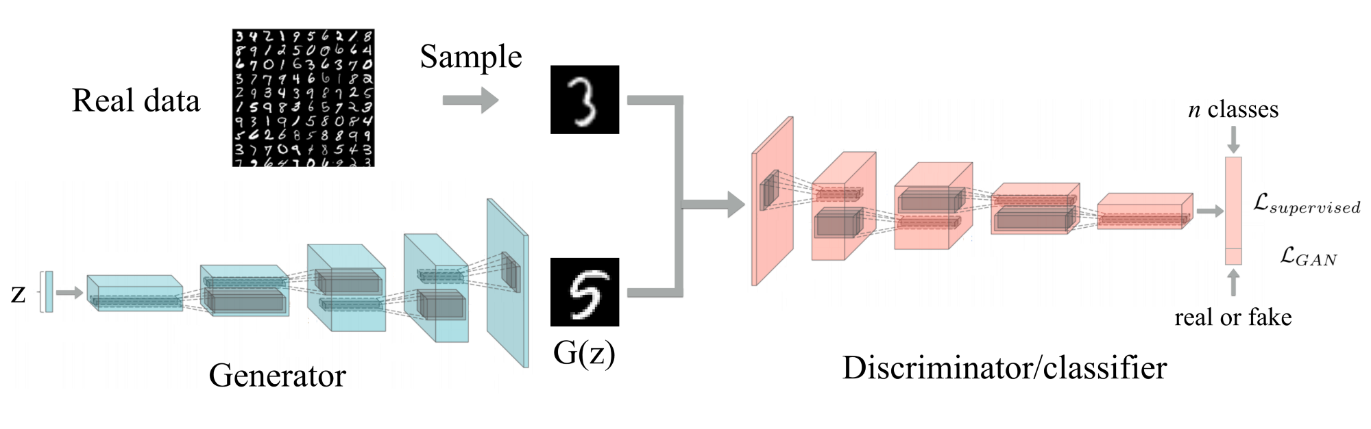

  For the semi-supervised task, in addition to R/F neuron, the discriminator will now have 10 more neurons for classification of MNIST digits. Also, this time their roles change and we can discard the generator after training, whose only objective was to generate unlabeled data to improve the discriminator’s performance.
  Now the discriminator is turned into an 11-class classifier with 1 neuron (R/F neuron) representing the fake data output and the other 10 representing real data with classes. The following has to be kept in mind:

• To assert R/F neuron output label = 0, when real unsupervised data from dataset is fed
• To assert R/F neuron output label= 1, when fake unsupervised data from generator is fed
• To assert R/F output label = 0 and corresponding label output = 1, when real supervised data is fed

This combination of different sources of data will help the discriminator classify more accurately than, if it had been only provided with a portion of labeled data.

Architecture

Now it’s time to get our hands dirty with some code :D
The Discriminator
  The architecture followed is similar to the one proposed in DCGAN paper. We use strided convolutions for reducing the dimensions of the feature-vectors rather than any pooling layers and apply a series of leaky_relu, dropout and BN for all layers to stabilize the learning. BN is dropped for input layer and last layer (for the purpose of feature matching). In the end, we perform Global Average Pooling to take the average over the spatial dimensions of the feature vectors. This squashes the tensor dimensions to a single value. After flattening the features, a dense layer of 11 classes is added with softmax activation for multi-class output.

1
2
3
4
5
6
7
8
9
10
11
12
13
14
15
16
17
18
19
20
21
22
23
24
25
26
27
28
29
30
31
32
33
34
35

def discriminator(x, dropout_rate = 0., is_training = True, reuse = False):
   # input x -> n+1 classes
   with tf.variable_scope('Discriminator', reuse = reuse): 
     # x = ?*64*64*1
     
     #Layer 1
     conv1 = tf.layers.conv2d(x, 128, kernel_size = [4,4], strides = [2,2],
                             padding = 'same', activation = tf.nn.leaky_relu, name = 'conv1') # ?*32*32*128
     #No batch-norm for input layer
     dropout1 = tf.nn.dropout(conv1, dropout_rate)
     
     #Layer2
     conv2 = tf.layers.conv2d(dropout1, 256, kernel_size = [4,4], strides = [2,2],
                             padding = 'same', activation = tf.nn.leaky_relu, name = 'conv2') # ?*16*16*256
     batch2 = tf.layers.batch_normalization(conv2, training = is_training)
     dropout2 = tf.nn.dropout(batch2, dropout_rate)
     
     #Layer3
     conv3 = tf.layers.conv2d(dropout2, 512, kernel_size = [4,4], strides = [4,4],
                             padding = 'same', activation = tf.nn.leaky_relu, name = 'conv3') # ?*4*4*512
     batch3 = tf.layers.batch_normalization(conv3, training = is_training)
     dropout3 = tf.nn.dropout(batch3, dropout_rate)
       
     # Layer 4
     conv4 = tf.layers.conv2d(dropout3, 1024, kernel_size=[3,3], strides=[1,1],
                              padding='valid',activation = tf.nn.leaky_relu, name='conv4') # ?*2*2*1024
     # No batch-norm as this layer's op will be used in feature matching loss
     # No dropout as feature matching needs to be definite on logits

     # Layer 5
     # Note: Applying Global average pooling        
     flatten = tf.reduce_mean(conv4, axis = [1,2])
     logits_D = tf.layers.dense(flatten, (1 + num_classes))
     out_D = tf.nn.softmax(logits_D)     
   return flatten,logits_D,out_D

The Generator
  The generator architecture is designed to mirror the discriminator’s spatial outputs. Fractional strided convolutions are used to increase the spatial dimension of the representation. An input of 4-D tensor of noise z is fed which undergoes a series of transposed convolutions, relu, BN(except at output layer) and dropout operations. Finally tanh activation maps the output image in range (-1,1).

1
2
3
4
5
6
7
8
9
10
11
12
13
14
15
16
17
18
19
20
21
22
23
24
25
26
27
28
29
30

def generator(z, dropout_rate = 0., is_training = True, reuse = False):
    # input latent z -> image x
    with tf.variable_scope('Generator', reuse = reuse):
      #Layer 1
      deconv1 = tf.layers.conv2d_transpose(z, 512, kernel_size = [4,4],
                                         strides = [1,1], padding = 'valid',
                                        activation = tf.nn.relu, name = 'deconv1') # ?*4*4*512
      batch1 = tf.layers.batch_normalization(deconv1, training = is_training)
      dropout1 = tf.nn.dropout(batch1, dropout_rate)
      
      #Layer 2
      deconv2 = tf.layers.conv2d_transpose(dropout1, 256, kernel_size = [4,4],
                                         strides = [4,4], padding = 'same',
                                        activation = tf.nn.relu, name = 'deconv2')# ?*16*16*256
      batch2 = tf.layers.batch_normalization(deconv2, training = is_training)
      dropout2 = tf.nn.dropout(batch2, dropout_rate)
        
      #Layer 3
      deconv3 = tf.layers.conv2d_transpose(dropout2, 128, kernel_size = [4,4],
                                         strides = [2,2], padding = 'same',
                                        activation = tf.nn.relu, name = 'deconv3')# ?*32*32*256
      batch3 = tf.layers.batch_normalization(deconv3, training = is_training)
      dropout3 = tf.nn.dropout(batch3, dropout_rate)
      
      #Output layer
      deconv4 = tf.layers.conv2d_transpose(dropout3, 1, kernel_size = [4,4],
                                        strides = [2,2], padding = 'same',
                                        activation = None, name = 'deconv4')# ?*64*64*1
      out = tf.nn.tanh(deconv4)
    return out

Model Loss

  We start by preparing an extended label for the whole batch by appending actual label to zeros. This is done to assert the R/F neuron output to 0 when the labeled data is fed. The discriminator loss for unlabeled data can be thought of as a binary sigmoid loss by asserting R/F neuron output to 1 for fake images and 0 for real images.

1
2
3
4
5
6
7
8
9
10
11
12
13
14
15
16
17
18
19

             ### Discriminator loss ###
# Supervised loss -> which class the real data belongs to    
temp = tf.nn.softmax_cross_entropy_with_logits_v2(logits = D_real_logit,
                                              labels = extended_label) 
# Labeled_mask and temp are of same size = batch_size where temp is softmax cross_entropy calculated over whole batch

D_L_Supervised = tf.reduce_sum(tf.multiply(temp,labeled_mask)) / tf.reduce_sum(labeled_mask)

# Multiplying temp with labeled_mask gives supervised loss on labeled_mask
# data only, calculating mean by dividing by no of labeled samples

# Unsupervised loss -> R/F    
D_L_RealUnsupervised = tf.reduce_mean(tf.nn.sigmoid_cross_entropy_with_logits(
        logits = D_real_logit[:, 0], labels = tf.zeros_like(D_real_logit[:, 0], dtype=tf.float32)))

D_L_FakeUnsupervised = tf.reduce_mean(tf.nn.sigmoid_cross_entropy_with_logits(
        logits = D_fake_logit[:, 0], labels = tf.ones_like(D_fake_logit[:, 0], dtype=tf.float32)))

D_L = D_L_Supervised + D_L_RealUnsupervised + D_L_FakeUnsupervised

  Generator loss is a combination of fake_image loss which falsely wants to assert R/F neuron output to 0 and feature matching loss which penalizes the mean absolute error between the average value of some set of features on the training data and the average values of that set of features on the generated samples.

1
2
3
4
5
6
7
8
9
10
11
12

             ### Generator loss ###                
# G_L_1 -> Fake data wanna be real 

G_L_1 = tf.reduce_mean(tf.nn.sigmoid_cross_entropy_with_logits(
        logits = D_fake_logit[:, 0],labels = tf.zeros_like(D_fake_logit[:, 0], dtype=tf.float32)))

# G_L_2 -> Feature matching
data_moments = tf.reduce_mean(D_real_features, axis = 0)
sample_moments = tf.reduce_mean(D_fake_features, axis = 0)
G_L_2 = tf.reduce_mean(tf.square(data_moments-sample_moments))

G_L = G_L_1 + G_L_2

Training

  The training images are resized from [batch_size, 28 ,28 , 1] to [batch_size, 64, 64, 1] to fit the generator/discriminator architectures. Losses, accuracies and generated samples are calculated and are observed to improve over each epoch.

1
2
3
4
5
6
7
8
9
10
11
12
13
14
15
16
17
18
19
20
21
22
23
24
25
26
27
28
29
30
31
32
33
34
35
36
37
38

for epoch in range(epochs):
  train_accuracies, train_D_losses, train_G_losses = [], [], []
  for it in range(no_of_batches):
  
  batch = mnist_data.train.next_batch(batch_size, shuffle = False)
  # batch[0] has shape: batch_size*28*28*1         
  batch_reshaped = tf.image.resize_images(batch[0], [64, 64]).eval()
  # Reshaping the whole batch into batch_size*64*64*1 for disc/gen architecture
  batch_z = np.random.normal(0, 1, (batch_size, 1, 1, latent))
  mask = get_labeled_mask(labeled_rate, batch_size)
                
  train_feed_dict = {x : scale(batch_reshaped), z : batch_z,
                              label : batch[1], labeled_mask : mask,
                               dropout_rate : 0.7, is_training : True}
  #The label provided in dict are one hot encoded in 10 classes
                
  D_optimizer.run(feed_dict = train_feed_dict)
  G_optimizer.run(feed_dict = train_feed_dict)
                
  train_D_loss = D_L.eval(feed_dict = train_feed_dict)
  train_G_loss = G_L.eval(feed_dict = train_feed_dict)
  train_accuracy = accuracy.eval(feed_dict = train_feed_dict)
          
  train_D_losses.append(train_D_loss)
  train_G_losses.append(train_G_loss)
  train_accuracies.append(train_accuracy)
          
  tr_GL = np.mean(train_G_losses)
  tr_DL = np.mean(train_D_losses)
  tr_acc = np.mean(train_accuracies)       
  
  print ('After epoch: '+ str(epoch+1) + ' Generator loss: '
                       + str(tr_GL) + ' Discriminator loss: ' + str(tr_DL) + ' Accuracy: ' + str(tr_acc))
        
  gen_samples = fake_data.eval(feed_dict = {z : np.random.normal(0, 1, (25, 1, 1, latent)), dropout_rate : 0.7, is_training : False})
  # Dont train batch-norm while plotting => is_training = False
  test_images = tf.image.resize_images(gen_samples, [64, 64]).eval()
  show_result(test_images, (epoch + 1), show = True, save = False, path = '')

Conclusion

  The training was done for 5 epochs and 20% labeled_rate due to restricted GPU access. For better results more training epochs with lesser labeled_rate is advised. The complete code notebook can be found here.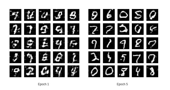

  Unsupervised learning is considered as a lacuna in the field of AGI. To bridge this gap, GANs are considered as a potential solution for learning complex tasks with low labeled data. With blooming new approaches in the domain of semi and unsupervised learning we can expect that this gap will lessen.
  I would be remiss not to mention my inspiration from this beautiful blog, this implementation along with the assistance of my colleague working on similar projects.
Until next time!! Kz

Reference

• Semi-Supervised Learning and GANs

引言

  本文主要介绍如何在tensorflow上仅使用200个带标签的mnist图像，实现在一万张测试图片上99%的测试精度，原理在于使用GAN做半监督学习。前文主要介绍一些原理部分，后文详细介绍代码及其实现原理。前文介绍比较简单，有基础的同学请略过直接看第二部分，文章末尾给出了代码GitHub链接。对GAN不了解的同学可以查看微信公众号：机器学习算法全栈工程师 的GAN入门文章。

1

本博客中的代码最终以GitHub中的代码为准，GitHub链接在文章底部，另外，本文已投稿至微信公众号：机器学习算法全栈工程师，欢迎关注此公众号

1.监督，无监督，半监督学习介绍

  在正式介绍实现半监督学习之前，我在这里首先介绍一下监督学习（supervised learning），半监督学习（semi-supervised learning）和无监督学习（unsupervised learning）的区别。

• 监督学习是指在训练集中包含训练数据的标签（label），比如类别标签，位置标签等等。最普遍使用标签学习的是分类任务，对于分类任务，输入给网络训练样本（samples）的一些特征（feature）以及此样本对应的标签（label），通过神经网络拟合的方法，神经网络可以在特征和标签之间找到一个合适的映射关系（mapping），这样当训练完成后，输入给网络没有label的样本，神经网络可以通过这一个映射关系猜出它属于哪一类。典型机器学习的监督学习的例子是KNN和SVM。目前机器视觉领域的急速发展离不开监督学习。
• 而无监督学习的训练事先没有训练标签，直接输入给算法一些数据，算法会努力学习数据的共同点，寻找样本之间的规律性。无监督学习是很典型的学习，人的学习有时候就是基于无监督的，比如我并不懂音乐，但是我听了上百首歌曲后，我可以根据我听的结果将音乐分为摇滚乐（记为0类）、民谣（记为1类）、纯音乐（记为2类）等等，事实上，我并不知道具体是哪一类，所以将它们记为0，1，2三类。典型的无监督学习方法是聚类算法，比如k-means。
• 东方快车电影里面大侦探有过一个台词，人们的话只有对与错，没有中间地带，最后经过一系列事件后他找到了对与错之间的betweeness。在监督学习和无监督学习之间，同样存在着中间地带——半监督学习。半监督学习简单来说就是将无监督学习和监督学习相结合，一部分包含了监督学习一部分包含了无监督学习，比如给一个分类任务，此分类任务的训练集中有精确标签的数据非常少，但是包含了大量的没有标注的数据，如果直接用监督学习的方法去做的话，效果不一定很好，有标注的训练数据太少很容易导致过拟合，而且大量的无标注的数据都没有充分的利用，最常见的例子是在医学图像的分析检测任务中，医学图像本身就不容易获得，要获得精标注的图像就需要有经验的医生去一个一个标注，显然他们并没有那么多的时间。这时候就是半监督学习的用武之地了，半监督学习很适合用在标签数据少，训练数据又比较多的情况。
  常见的半监督学习方法主要有：
    1.Self training
    2.Generative model
    3.S3VMs
    4.Graph-Based AIgorithems
    5.Multiview AIgorithems

  接下来我会结合Improved Techniques for Training GANs这篇论文详细介绍如何使用目前最火的生成对抗模型GAN去实现半监督学习，也即是半监督学习的第二种方法，并给出详细的代码解释，对理论不是很熟悉的同学可以直接看代码。另外注明：我只复现了论文半监督学习的部分，之前也有人复现了此部分，但是我感觉他对原文有很大的曲解，他使用了所有的标签去帮助生成，并不在分类上，不太符合半监督学习的本质，而且代码很复杂，感兴趣的可以去GitHub上搜ssgan,希望能帮助你。

2. Improved Techniques for Training GANs

  GAN是无监督学习的代表，它可以不断学习模拟数据的分布进而生成和训练数据相似分布的样本，在训练过程不需要标签，GAN在无监督学习领域，生成领域，半监督学习领域以及强化学习领域都有广泛的应用。但是GAN存在很多的训练不稳定等等的问题，作者good fellow在2016年放出了Improved Techniques for Training GANs，对GAN训练不稳定的问题做了一些解释和经验上的解决方案，并给出了和半监督学习结合的方法。
  从平衡点角度解释GAN的不稳定性来说，GAN的纳什均衡点是一个鞍点，并不是一个局部最小值点，基于梯度的方法主要是寻找高维空间中的极小值点，因此使用梯度训练的方法很难使GAN收敛到平衡点。为此，为了进一部分缓解这个问题，goodfellow联合提出了一些改进方案，
主要有：

• Feature matching,
• Minibatch discrimination
• weight Historical averaging (相当于一个正则化的方式)
• One-sided label smoothing
• Virtual batch normalization

后来发现Feature matching在半监督学习上表现良好，mini-batch discrimination表现很差。

3. semi-supervised GAN

  对于一个普通的分类器来说，假设对MNIST分类，一共有10类数据，分别是0-9，分类器模型以数据x作为输入，输出一个K=10维的向量，经过softmax后计算出分类概率最大的那个类别。在监督学习领域，往往是通过最小化类别标签和预测分布 的交叉熵来实现最好的结果。
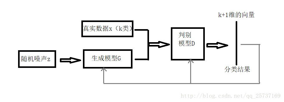
  但是将GAN用在半监督学习领域的时候需要做一些改变，生成器不做改变，仍然负责从输入噪声数据中生成图像，判别器D不在是一个简单的真假分类（二分类）器，假设输入数据有K类，D就是K+1的分类器，多出的那一类是判别输入是否是生成器G生成的图像。网络的流程图见下图：

  网络结构确定了之后就是损失函数的设计部分，借助GAN我们就可以从无标签数据中学习，只要知道输入数据是真实数据，那就可以通过最大化\(logP_{model}(y\in{1,2,…,K}|x)\)来实现，上述式子可解释为不管输入的是哪一类真的图片（不是生成器G生成的假图片），只要最大化输出它是真图像的概率就可以了，不需要具体分出是哪一类。由于GAN的生成器的参与，训练数据中有一半都是生成的假数据。
  下面给出判别器D的损失函数设计，D损失函数包括两个部分，一个是监督学习损失，一个是半监督学习损失，具体公式如下：

其中：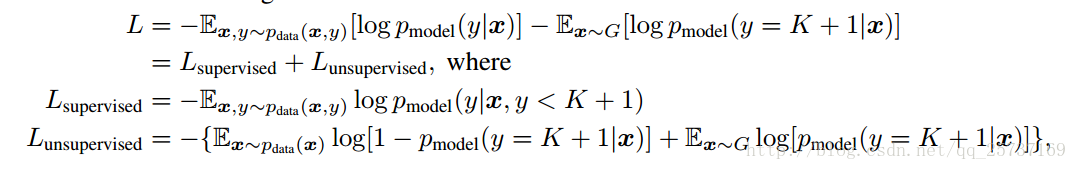

对于无监督学习来说，只需要输出真假就可以了，不需要确定是哪一类，因此我们令

其中\( P_{model} \)表示判别是假图像的概率，那么D(x)就代表了输出是真图像的概率，那么无监督学习的损失函数就可以表示为

  这不就是GAN的损失函数嘛！好了，到这里得出结论，在半监督学习中，判别器的分类要多分一类，多出的这一类表示的是生成器生成的假图像这一类，另外判别器的损失函数不仅包括了监督损失函数而且还有无监督的损失函数，在训练过程中同时最小化这两者。损失函数介绍完毕，接下来介绍代码实现部分。

4.代码实现及解读

  注：完整代码的GitHub连接在文章底部。这里只截取关键部分做介绍
  在代码中，我使用feature matching，one side label smoothing方式，并没有使用论文中介绍的Historical averaging,而是只对判别器D使用了简单的l2正则化，防止过拟合，另外论文中介绍的Minibatch discrimination, Virtual batch normalization等等都没有使用，主要是这两者在半监督学习中表现不是很好，但是如果想获得好的生成结果还是很有用的。
  首先介绍网络结构部分，因为是在mnist数据集比较简单，所以随便搭了一个判别器和生成器，具体如下：

1
2
3
4
5
6
7
8
9
10
11
12
13
14
15
16
17
18
19
20
21
22

def discriminator(self, name, inputs, reuse):
        l = tf.shape(inputs)[0]
        inputs = tf.reshape(inputs, (l,self.img_size,self.img_size,self.dim))
        with tf.variable_scope(name,reuse=reuse):
            out = []
            output = conv2d('d_con1',inputs,5, 64, stride=2, padding='SAME') #14*14
            output1 = lrelu(self.bn('d_bn1',output))
            out.append(output1)
            # output1 = tf.contrib.keras.layers.GaussianNoise
            output = conv2d('d_con2', output1, 3, 64*2, stride=2, padding='SAME')#7*7
            output2 = lrelu(self.bn('d_bn2', output))
            out.append(output2)
            output = conv2d('d_con3', output2, 3, 64*4, stride=1, padding='VALID')#5*5
            output3 = lrelu(self.bn('d_bn3', output))
            out.append(output3)
            output = conv2d('d_con4', output3, 3, 64*4, stride=2, padding='VALID')#2*2
            output4 = lrelu(self.bn('d_bn4', output))
            out.append(output4)
            output = tf.reshape(output4, [l, 2*2*64*4])# 2*2*64*4
            output = fc('d_fc', output, self.num_class)
            # output = tf.nn.softmax(output)
            return output, out

  其中conv2d()是卷积操作，参数依次是，层的名字，输入tensor，卷积核大小，输出通道数，步长，padding。判别器中每一层都加了归一化层，这里使用最简单的归一化，函数如下所示，另外每一层的激活函数使用leakyrelu。判别器D最终返回两个值，第一个是计算的logits，另外一个是一个列表，列表的每一个元素代表判别器每一层的输出，为接下来实现feature matching做准备。
  生成器结构如下所示：其最后一层激活函数使用tanh

1
2
3
4
5
6
7
8
9
10
11
12
13
14
15
16
17
18
19

def generator(self,name, noise, reuse):
    with tf.variable_scope(name,reuse=reuse):
        l = self.batch_size
        output = fc('g_dc', noise, 2*2*64)
        output = tf.reshape(output, [-1, 2, 2, 64])
        output = tf.nn.relu(self.bn('g_bn1',output))
        output = deconv2d('g_dcon1',output,5,outshape=[l, 4, 4, 64*4])
        output = tf.nn.relu(self.bn('g_bn2',output))

        output = deconv2d('g_dcon2', output, 5, outshape=[l, 8, 8, 64 * 2])
        output = tf.nn.relu(self.bn('g_bn3', output))

        output = deconv2d('g_dcon3', output, 5, outshape=[l, 16, 16,64 * 1])
        output = tf.nn.relu(self.bn('g_bn4', output))

        output = deconv2d('g_dcon4', output, 5, outshape=[l, 32, 32, self.dim])
        output = tf.image.resize_images(output, (28, 28))
        # output = tf.nn.relu(self.bn('g_bn4', output))
        return tf.nn.tanh(output)

网络结构是根据DCGAN的结构改的，所以网络简要介绍到这里。

接下来介绍网络初始化方面：
首先在train.py里建立一个Train的类，并做一些初始化

1
2
3
4
5
6
7
8
9
10
11
12
13
14
15
16
17
18
19
20
21
22
23
24
25
26
27
28
29
30
31
32
33
34
35
36
37
38
39
40
41
42
43
44
45
46
47
48
49
50
51
52
53
54
55
56
57
58
59
60
61
62
63
64
65
66
67
68
69
70
71
72
73
74
75
76
77
78
79
80
81
82
83
84
85
86
87
88
89
90
91
92
93
94
95
96
97
98
99
100
101
102
103
104
105
106
107
108
109
110
111
112
113
114
115
116
117
118
119
120
121
122
123
124
125
126
127
128
129
130
131
132
133
134
135
136
137
138
139
140
141
142
143
144
145
146
147
148
149
150
151
152
153
154
155
156
157
158
159
160
161
162
163
164
165
166
167
168
169
170
171
172
173
174
175
176
177
178
179
180
181
182
183
184
185
186
187
188
189
190
191
192
193
194
195
196
197
198
199
200
201
202
203
204
205
206
207
208
209
210
211
212
213
214
215

#coding:utf-8
from glob import glob
from PIL import Image
import matplotlib.pyplot as plt
import scipy.misc as scm
from vlib.layers import *
import tensorflow as tf
import numpy as np
from vlib.load_data import *
import os
import vlib.plot as plot
import vlib.my_extract as dataload
import vlib.save_images as save_img
import time
from tensorflow.examples.tutorials.mnist import input_data #as mnist_data
mnist = input_data.read_data_sets('data/', one_hot=True)
# temp = 0.89
class Train(object):
    def __init__(self, sess, args):
        #sess=tf.Session()
        self.sess = sess
        self.img_size = 28   # the size of image
        self.trainable = True
        self.batch_size = 50  # must be even number
        self.lr = 0.0002
        self.mm = 0.5      # momentum term for adam
        self.z_dim = 128   # the dimension of noise z
        self.EPOCH = 50    # the number of max epoch
        self.LAMBDA = 0.1  # parameter of WGAN-GP
        self.model = args.model  # 'DCGAN' or 'WGAN'
        self.dim = 1       # RGB is different with gray pic
        self.num_class = 11
        self.load_model = args.load_model
        self.build_model()  # initializer

    def build_model(self):
        # build  placeholders
        self.x=tf.placeholder(tf.float32,shape=[self.batch_size,self.img_size*self.img_size*self.dim],name='real_img')
        self.z = tf.placeholder(tf.float32, shape=[self.batch_size, self.z_dim], name='noise')
        self.label = tf.placeholder(tf.float32, shape=[self.batch_size, self.num_class - 1], name='label')
        self.flag = tf.placeholder(tf.float32, shape=[], name='flag')
        self.flag2 = tf.placeholder(tf.float32, shape=[], name='flag2')

        # define the network
        self.G_img = self.generator('gen', self.z, reuse=False)
        d_logits_r, layer_out_r = self.discriminator('dis', self.x, reuse=False)
        d_logits_f, layer_out_f = self.discriminator('dis', self.G_img, reuse=True)

        d_regular = tf.add_n(tf.get_collection('regularizer', 'dis'), 'loss')  # D regular loss
        # caculate the unsupervised loss
        un_label_r = tf.concat([tf.ones_like(self.label), tf.zeros(shape=(self.batch_size, 1))], axis=1)
        un_label_f = tf.concat([tf.zeros_like(self.label), tf.ones(shape=(self.batch_size, 1))], axis=1)
        logits_r, logits_f = tf.nn.softmax(d_logits_r), tf.nn.softmax(d_logits_f)
        d_loss_r = -tf.log(tf.reduce_sum(logits_r[:, :-1])/tf.reduce_sum(logits_r[:,:]))
        d_loss_f = -tf.log(tf.reduce_sum(logits_f[:, -1])/tf.reduce_sum(logits_f[:,:]))
        # d_loss_r = tf.reduce_mean(tf.nn.softmax_cross_entropy_with_logits(labels=un_label_r*0.9, logits=d_logits_r))
        # d_loss_f = tf.reduce_mean(tf.nn.softmax_cross_entropy_with_logits(labels=un_label_f*0.9, logits=d_logits_f))
        # feature match
        f_match = tf.constant(0., dtype=tf.float32)
        for i in range(4):
            f_match += tf.reduce_mean(tf.multiply(layer_out_f[i]-layer_out_r[i], layer_out_f[i]-layer_out_r[i]))

        # caculate the supervised loss
        s_label = tf.concat([self.label, tf.zeros(shape=(self.batch_size,1))], axis=1)
        s_l_r = tf.reduce_mean(tf.nn.softmax_cross_entropy_with_logits(labels=s_label*0.9, logits=d_logits_r))
        s_l_f = tf.reduce_mean(tf.nn.softmax_cross_entropy_with_logits(labels=un_label_f*0.9, logits=d_logits_f))  # same as d_loss_f
        self.d_l_1, self.d_l_2 = d_loss_r + d_loss_f, s_l_r
        self.d_loss = d_loss_r + d_loss_f + s_l_r*self.flag*10 + d_regular
        self.g_loss = d_loss_f + 0.01*f_match

        all_vars = tf.global_variables()
        g_vars = [v for v in all_vars if 'gen' in v.name]
        d_vars = [v for v in all_vars if 'dis' in v.name]
        for v in all_vars:
            print v
        if self.model == 'DCGAN':
            self.opt_d = tf.train.AdamOptimizer(self.lr, beta1=self.mm).minimize(self.d_loss, var_list=d_vars)
            self.opt_g = tf.train.AdamOptimizer(self.lr, beta1=self.mm).minimize(self.g_loss, var_list=g_vars)
        elif self.model == 'WGAN_GP':
            self.opt_d = tf.train.AdamOptimizer(1e-5, beta1=0.5, beta2=0.9).minimize(self.d_loss, var_list=d_vars)
            self.opt_g = tf.train.AdamOptimizer(1e-5, beta1=0.5, beta2=0.9).minimize(self.g_loss, var_list=g_vars)
        else:
            print ('model can only be "DCGAN","WGAN_GP" !')
            return
        # test
        test_logits, _ = self.discriminator('dis', self.x, reuse=True)
        test_logits = tf.nn.softmax(test_logits)
        temp = tf.reshape(test_logits[:, -1],shape=[self.batch_size, 1])
        for i in range(10):
            temp = tf.concat([temp, tf.reshape(test_logits[:, -1],shape=[self.batch_size, 1])], axis=1)
        test_logits -= temp
        self.prediction = tf.nn.in_top_k(test_logits, tf.argmax(s_label, axis=1), 1)

        self.saver = tf.train.Saver()
        if not self.load_model:
            init = tf.global_variables_initializer()
            self.sess.run(init)
        elif self.load_model:
            self.saver.restore(self.sess, os.getcwd()+'/model_saved/model.ckpt')
            print 'model load done'
        self.sess.graph.finalize()

    def train(self):
        if not os.path.exists('model_saved'):
            os.mkdir('model_saved')
        if not os.path.exists('gen_picture'):
            os.mkdir('gen_picture')
        noise = np.random.normal(-1, 1, [self.batch_size, 128])
        temp = 0.80
        print 'training'
        for epoch in range(self.EPOCH):
            # iters = int(156191//self.batch_size)
            iters = 50000//self.batch_size
            flag2 = 1  # if epoch>10 else 0
            for idx in range(iters):
                start_t = time.time()
                flag = 1 if idx < 4 else 0 # set we use 2*batch_size=200 train data labeled.
                batchx, batchl = mnist.train.next_batch(self.batch_size)
                # batchx, batchl = self.sess.run([batchx, batchl])
                g_opt = [self.opt_g, self.g_loss]
                d_opt = [self.opt_d, self.d_loss, self.d_l_1, self.d_l_2]
                feed = {self.x:batchx, self.z:noise, self.label:batchl, self.flag:flag, self.flag2:flag2}
                # update the Discrimater k times
                _, loss_d, d1,d2 = self.sess.run(d_opt, feed_dict=feed)
                # update the Generator one time
                _, loss_g = self.sess.run(g_opt, feed_dict=feed)
                print ("[%3f][epoch:%2d/%2d][iter:%4d/%4d],loss_d:%5f,loss_g:%4f, d1:%4f, d2:%4f"%
                       (time.time()-start_t, epoch, self.EPOCH,idx,iters, loss_d, loss_g,d1,d2)), 'flag:',flag
                plot.plot('d_loss', loss_d)
                plot.plot('g_loss', loss_g)
                if ((idx+1) % 100) == 0:  # flush plot picture per 1000 iters
                    plot.flush()
                plot.tick()
                if (idx+1)%500==0:
                    print ('images saving............')
                    img = self.sess.run(self.G_img, feed_dict=feed)
                    save_img.save_images(img, os.getcwd()+'/gen_picture/'+'sample{}_{}.jpg'\
                                         .format(epoch, (idx+1)/500))
                    print 'images save done'
            test_acc = self.test()
            plot.plot('test acc', test_acc)
            plot.flush()
            plot.tick()
            print 'test acc:{}'.format(test_acc), 'temp:%3f'%(temp)
            if test_acc > temp:
                print ('model saving..............')
                path = os.getcwd() + '/model_saved'
                save_path = os.path.join(path, "model.ckpt")
                self.saver.save(self.sess, save_path=save_path)
                print ('model saved...............')
                temp = test_acc

# output = conv2d('Z_cona{}'.format(i), output, 3, 64, stride=1, padding='SAME')

    def generator(self,name, noise, reuse):
        with tf.variable_scope(name,reuse=reuse):
            l = self.batch_size
            output = fc('g_dc', noise, 2*2*64)
            output = tf.reshape(output, [-1, 2, 2, 64])
            output = tf.nn.relu(self.bn('g_bn1',output))
            output = deconv2d('g_dcon1',output,5,outshape=[l, 4, 4, 64*4])
            output = tf.nn.relu(self.bn('g_bn2',output))

            output = deconv2d('g_dcon2', output, 5, outshape=[l, 8, 8, 64 * 2])
            output = tf.nn.relu(self.bn('g_bn3', output))

            output = deconv2d('g_dcon3', output, 5, outshape=[l, 16, 16,64 * 1])
            output = tf.nn.relu(self.bn('g_bn4', output))

            output = deconv2d('g_dcon4', output, 5, outshape=[l, 32, 32, self.dim])
            output = tf.image.resize_images(output, (28, 28))
            # output = tf.nn.relu(self.bn('g_bn4', output))
            return tf.nn.tanh(output)

    def discriminator(self, name, inputs, reuse):
        l = tf.shape(inputs)[0]
        inputs = tf.reshape(inputs, (l,self.img_size,self.img_size,self.dim))
        with tf.variable_scope(name,reuse=reuse):
            out = []
            output = conv2d('d_con1',inputs,5, 64, stride=2, padding='SAME') #14*14
            output1 = lrelu(self.bn('d_bn1',output))
            out.append(output1)
            # output1 = tf.contrib.keras.layers.GaussianNoise
            output = conv2d('d_con2', output1, 3, 64*2, stride=2, padding='SAME')#7*7
            output2 = lrelu(self.bn('d_bn2', output))
            out.append(output2)
            output = conv2d('d_con3', output2, 3, 64*4, stride=1, padding='VALID')#5*5
            output3 = lrelu(self.bn('d_bn3', output))
            out.append(output3)
            output = conv2d('d_con4', output3, 3, 64*4, stride=2, padding='VALID')#2*2
            output4 = lrelu(self.bn('d_bn4', output))
            out.append(output4)
            output = tf.reshape(output4, [l, 2*2*64*4])# 2*2*64*4
            output = fc('d_fc', output, self.num_class)
            # output = tf.nn.softmax(output)
            return output, out

    def bn(self, name, input):
        val = tf.contrib.layers.batch_norm(input, decay=0.9,
                                           updates_collections=None,
                                           epsilon=1e-5,
                                           scale=True,
                                           is_training=True,
                                           scope=name)
        return val

    # def get_loss(self, logits, layer_out):
    def test(self):
        count = 0.
        print 'testing................'
        for i in range(10000//self.batch_size):
            testx, textl = mnist.test.next_batch(self.batch_size)
            prediction = self.sess.run(self.prediction, feed_dict={self.x:testx, self.label:textl})
            count += np.sum(prediction)
        return count/10000.

  args是传进来的参数，主要包括三个，

• 一个是args.model，选择DCGAN模式还是WGAN-GP模式，二者的不同主要在于损失函数不同和优化器的学习率不同，其他都一样。
• 第二个参数是args.trainable，训练还是测试，训练时为True，测试是False。
• Loadmodel表示是否选择加载训练好的权重。

  Build_model函数里面主要包括了网络训练前的准备工作，主要包括损失函数的设计和优化器的设计。下文将详细做出介绍，尤其是损失函数部分。
  首先，建立了五个placeholder，flag表示两个标志位，只有0-1两种情况，注意到我num_class是11，也就是做11分类，但是lable的placeholder中shape是(batchsize,10)。为了方便，我将生成器的生成结果和真实数据X级联在一起作为判别器的输入，输出再把他它们结果split分开。
  d_regular 表示正则化，这里我将判别器中所有的weights做了l2正则。
  监督学习的损失函数使用常见的交叉熵损失函数，对生成器生成的图像的label的one_hot型为：
[0, 0, 0, 0, 0, 0, 0, 0, 0, 0, 1]
  将原始的label扩展到(batchsize，11)后再和生成器生成的假数据的label在第一维度concat到一起得到batchl，另外乘以0.9，做单边标签平滑（one side smoothing），由此计算得到监督学习的损失函数值s_l,。

生成器G的损失函数

  生成器G的损失函数包括两部分，一个是来自GAN训练的部分，另外一个是feature matching , 论文中提到的feature matching意思是特征匹配，主要思想是希望生成器生成的假数据输入到判别器，经过判别器每一层计算的结果和将真实数据X输入到判别器，判别器每一层的结果尽可能的相似，公式如下：

  其中\(f(x)\)是D的每一层的输出。Feature matching 是指导G进行训练，所以我将他放在了G的损失函数里。

分类器D的损失函数：

相比较G的损失函数，D的损失函数就比较麻烦了
接下来介绍无监督学习的损失函数实现：
在前面介绍的无监督学习的损失函数中，有一部分和GAN的损失函数很相似，所以在代码中我们使用了

  无监督学习的时候没有标签的指导，此时判别器或者称为分类器D无法正确对输入进行分类，此时只要求D能够区分真假就可以了，由此我们得到了无监督学习的损失un_s，直观上也很好理解，假设输入给判别器D真图像，它结果经过softmax后输出类似下面表格的形式，其中前十个黄色区域表示对0-9的分类概率，最后一个灰色的表示对假图像的分类概率，由于无监督学习中判别器D并不知道具体是哪一类数据，所以干脆D的损失函数最小化输出假图像的概率就可以了，当输入为生成器生成的假图像时，只要最小化D输出为真图像的概率，由此我们得到了un_s.。但是此时有一个问题，即是有监督学习的时候不就没有用了吗，因为这时候应该使用s_l.为了解决这个问题，我使用了一个标志位flag作为控制他们之间的使用，具体代码：

  有标签的时候flag是1，表示使用s_l,无监督的时候flag是0，表示使用无监督损失函数。此时已经完成了判别器D损失函数的一部分设计，剩下的一部分和GAN中的D的损失一样，在代码中我给出了两种损失函数，一个是原始GAN的交叉熵损失函数，和DCGAN使用的一样，另外一个是improved wgan论文中使用的损失函数，但是在做了对比之后，我强烈建议使用DCGAN来做，improved wgan的损失函数虽然在生成结果的优化上有很大帮助，但是并不适合半监督学习中。

训练

接下来就是训练部分：
  此时可能有一个疑问，我们是如何实现只使用200带标签的数据训练的，答案就在flag这个标志位里，在训练部分代码中，当迭代次数小于200的时候，flag=1, 此时表示使用s_l作为损失函数的一部分，当flag=0的时候，un_s起作用而s_l并没有起作用，这时，即使我们feed了正确的标签数据，但是s_l不起作用，就相当于没有使用标签。
  flag的作用本来是使用他控制feature matching是否工作的，因为这部分损失相当的大，后来发现影响不大，暂时就放在这里了。

测试

1
2
3
4
5
6
7
8

def test(self):
       count = 0.
       print 'testing................'
       for i in range(10000//self.batch_size):
           testx, textl = mnist.test.next_batch(self.batch_size)
           prediction = self.sess.run(self.prediction, feed_dict={self.x:testx, self.label:textl})
           count += np.sum(prediction)
       return count/10000.

测试精度结果变化图

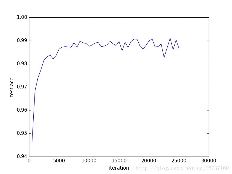
本文实验代码

使用GAN实现半监督学习代码https://github.com/LDOUBLEV/semi-supervised-GAN
如果感觉有用的话，欢迎star， fork

备注

  详细代码请以github中为准，另关于结果不理想的问题，可能和之前做的迁移学习有关，下面是最近跑出来的结果，最好的精度是0.95，这个问题有时间会慢慢解决。另：链接中的模型精度是很高的，可以直接调用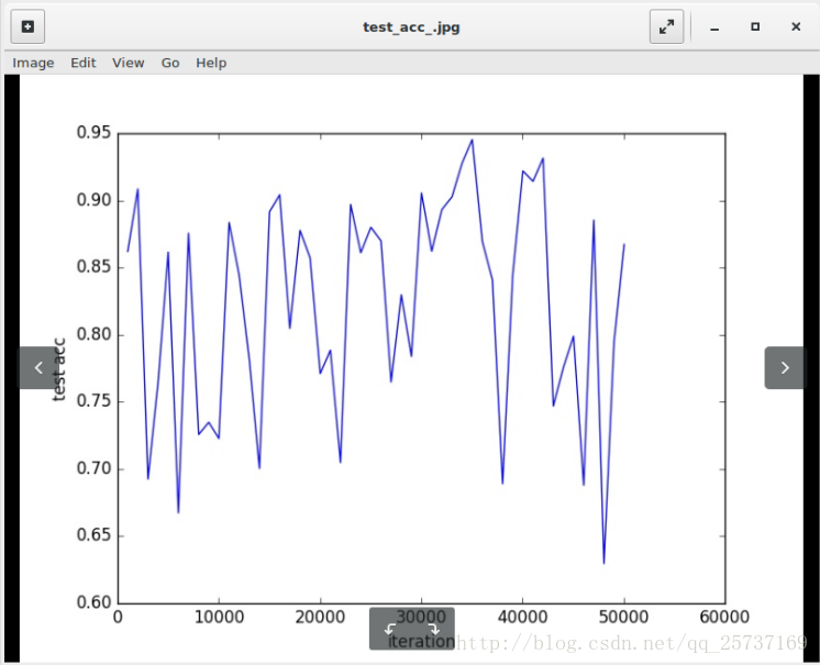

参考文献

• 手把手教你用GAN实现半监督学习

TensorFlowSharp安装和使用入门

(posted @ 2017-11-25 21:31)
Tensorflow是一个人工智能框架。TensorflowSharp是对Tensorflow C语言版接口的封装，便于C#开发人员在项目中使用Tensorflow。

一、使用方法

TensorflowSharp的使用很简单，首先使用NuGet安装TensorflowSharp包，然后新建C#控制台程序，输入下面代码，运行即可。

1
2
3
4
5
6
7
8
9
10
11
12
13
14
15
16
17
18
19
20
21
22
23
24

// 创建图
var g = new TFGraph();

// 定义常量
var a = g.Const(2);
var b = g.Const(3);

// 加法和乘法运算
var add = g.Add(a, b);
var mul = g.Mul(a, b);

// 创建会话
var sess = new TFSession(g);

// 计算加法
var result1 = sess.GetRunner().Run(add).GetValue();
Console.WriteLine("a+b={0}", result1);

// 计算乘法
var result2 = sess.GetRunner().Run(mul).GetValue();
Console.WriteLine("a*b={0}", result2);

// 关闭会话
sess.CloseSession();

运行后输出结果：

1
2

a+b=5
a*b=6

二、注意事项

1. 国内目前无法访问Tensorflow官网，但是可以访问谷歌提供的Tensorflow官网镜像。
2. 国内使用NuGet安装TensorflowSharp很容易失败，可以直接从Nuget官网下载，然后改后缀名zip，解压后手工安装。
3. TensorflowSharp项目使用的.net版本必须高于4.6.1，本教程使用的版本是4.7.0，可以在属性选项卡中设置。
4. TensorflowSharp项目必须使用64位CPU，需要在属性选项卡生成中，去掉首选32位的勾选。
5. 手动安装TensorflowSharp，处理要引用TensorFlowSharp.dll，还要将libtensorflow.dll复制到每个项目的输出目录。

三、相关网站

Tensorflow教程：https://github.com/tengge1/learn-tensorflow-sharp
Tensorflow官网：http://www.tensorflow.org
Google Tensorflow镜像：https://tensorflow.google.cn/
Tensorflow开源项目：https://github.com/tensorflow/tensorflow
TensorflowSharp开源项目：https://github.com/migueldeicaza/TensorFlowSharp
TensorflowSharp NuGet主页：https://www.nuget.org/packages/TensorFlowSharp/
Tensorflow中文社区：http://www.tensorfly.cn/

03 使用TensorFlow做计算题

我们使用Tensorflow，计算((a+b)*c)^2/a，然后求平方根。看代码：

1
2
3
4
5
6
7
8
9
10
11
12
13
14
15
16
17
18
19
20
21
22
23
24
25
26
27
28

import tensorflow as tf

# 输入储存容器
a = tf.placeholder(tf.float16)
b = tf.placeholder(tf.float16)
c = tf.placeholder(tf.float16)

# 计算
d = tf.add(a, b) #加法
e = tf.multiply(d, c) #乘法
f = tf.pow(e, 2) #平方
g = tf.divide(f, a) #除法
h = tf.sqrt(g) #平方根

# 会话
sess = tf.Session()

# 赋值
feed_dict= {a:1, b:2, c:3}

# 计算
result = sess.run(h, feed_dict= feed_dict)

# 关闭会话
sess.close()

# 输出结果
print(result)

这里让a=1，b=2，c=3，如果输出9.0，证明运行成功。
Tensorflow做计算的方法是，先把计算的式子构建一个图，然后把这个图和赋值在cpu上一起运行，计算速度比较快。

04 TensorFlow中的常量、变量和数据类型

打开Python Shell，先输入import tensorflow as tf，然后可以执行以下命令。
Tensorflow中的常量创建方法：

1

hello = tf.constant('Hello,world!', dtype=tf.string)

其中，’Hello,world!’是常量初始值；tf.string是常量类型，可以省略。常量和变量都可以去构建Tensorflow中的图。

Tensorflow中变量的创建方法：

1

a = tf.Variable(10, dtype=tf.int32)

其中，10是变量初始值，tf.int32是变量的类型。
Tensorflow中，主要有以下几种数据类型。
tf.int8：8位整数。
tf.int16：16位整数。
tf.int32：32位整数。
tf.int64：64位整数。

tf.uint8：8位无符号整数。
tf.uint16：16位无符号整数。

tf.float16：16位浮点数。
tf.float32：32位浮点数。
tf.float64：64位浮点数。
tf.double：等同于tf.float64。

tf.string：字符串。

tf.bool：布尔型。

tf.complex64：64位复数。
tf.complex128：128位复数。

参考文献

• 《张量的阶、形状、数据类型》

05 TensorFlow中变量的初始化

打开Python Shell，输入import tensorflow as tf，然后可以执行以下代码。
1、创建一个2*3的矩阵，并让所有元素的值为0.（类型为tf.float）

1

a = tf.zeros([2,3], dtype = tf.float32)

2、创建一个3*4的矩阵，并让所有元素的值为1.

1

b = tf.ones([3,4])

3、创建一个1*10的矩阵，使用2来填充。（类型为tf.int32，可忽略）

1

c = tf.constant(2, dtype=tf.int32, shape=[1,10])

4、创建一个1*10的矩阵，其中的元素符合正态分布，平均值是20，标准偏差是3.

1

d = tf.random_normal([1,10],mean = 20, stddev = 3)

上面所有的值都可以用来初始化变量。例如用0.01来填充一个1*2的矩阵来初始化一个叫bias的变量。

1

bias = tf.Variable(tf.zeros([1,2]) + 0.01)

如果你想查看这些量具体的值，可以在Session中执行它并输出。

1
2

sess = tf.Session()
print(sess.run(d))

这里，我得到了以下的值：
[[ 22.44503784 18.19544983 17.89671898 17.67314911 19.45074844
18.6805439 18.56541443 16.59041977 22.11240005 19.12819099]]。它就是上面4我们创建的量的值。

参考文献

• 《Tensorflow学习笔记（3）》

06 使用TensorFlow拟合x与y之间的关系

看代码：

1
2
3
4
5
6
7
8
9
10
11
12
13
14
15
16
17
18
19
20
21
22
23
24
25
26
27
28
29
30
31
32
33
34
35
36
37
38

import tensorflow as tf
import numpy as np

#构造输入数据（我们用神经网络拟合x_data和y_data之间的关系）
x_data = np.linspace(-1,1,300)[:, np.newaxis] #-1到1等分300份形成的二维矩阵
noise = np.random.normal(0,0.05, x_data.shape) #噪音，形状同x_data在0-0.05符合正态分布的小数
y_data = np.square(x_data)-0.5+noise #x_data平方，减0.05，再加噪音值

#输入层（1个神经元）
xs = tf.placeholder(tf.float32, [None, 1]) #占位符，None表示n*1维矩阵，其中n不确定
ys = tf.placeholder(tf.float32, [None, 1]) #占位符，None表示n*1维矩阵，其中n不确定

#隐层（10个神经元）
W1 = tf.Variable(tf.random_normal([1,10])) #权重，1*10的矩阵，并用符合正态分布的随机数填充
b1 = tf.Variable(tf.zeros([1,10])+0.1) #偏置，1*10的矩阵，使用0.1填充
Wx_plus_b1 = tf.matmul(xs,W1) + b1 #矩阵xs和W1相乘，然后加上偏置
output1 = tf.nn.relu(Wx_plus_b1) #激活函数使用tf.nn.relu

#输出层（1个神经元）
W2 = tf.Variable(tf.random_normal([10,1]))
b2 = tf.Variable(tf.zeros([1,1])+0.1)
Wx_plus_b2 = tf.matmul(output1,W2) + b2
output2 = Wx_plus_b2

#损失
loss = tf.reduce_mean(tf.reduce_sum(tf.square(ys-output2),reduction_indices=[1])) #在第一维上，偏差平方后求和，再求平均值，来计算损失
train_step = tf.train.GradientDescentOptimizer(0.1).minimize(loss) # 使用梯度下降法，设置步长0.1，来最小化损失

#初始化
init = tf.global_variables_initializer() #初始化所有变量
sess = tf.Session()
sess.run(init) #变量初始化

#训练
for i in range(1000): #训练1000次
    _,loss_value = sess.run([train_step,loss],feed_dict={xs:x_data,ys:y_data}) #进行梯度下降运算，并计算每一步的损失
    if(i%50==0):
        print(loss_value) # 每50步输出一次损失

输出：
0.405348
0.00954485
0.0068925
0.00551958
0.00471453
0.00425206
0.00400382
0.00381883
0.00367445
0.00353349
0.00341325
0.00330487
0.00321128
0.00313468
0.0030646
0.0030014
0.00294802
0.00290179
0.0028618
0.00282344
可以看到，随机训练的进行，损失越来越小，证明拟合越来越好。

参考文献

1. 《Tensorflow 自带可视化Tensorboard使用方法 附项目代码》
2. 《tensorflow学习（六）：tensorflow中的tf.reduce_mean()这类函数》

07 训练TensorFlow识别手写数字

打开Python Shell，输入以下代码：

1
2
3
4
5
6
7
8
9
10
11
12
13
14
15
16
17
18
19
20
21
22
23
24
25
26
27
28
29
30
31
32
33
34

import tensorflow as tf
from tensorflow.examples.tutorials.mnist import input_data

# 获取数据（如果存在就读取，不存在就下载完再读取）
mnist = input_data.read_data_sets("MNIST_data/", one_hot=True)

# 输入
x = tf.placeholder("float", [None, 784]) #输入占位符（每张手写数字784个像素点）
y_ = tf.placeholder("float", [None,10]) #输入占位符（这张手写数字具体代表的值，0-9对应矩阵的10个位置）

# 计算分类softmax会将xW+b分成10类，对应0-9
W = tf.Variable(tf.zeros([784,10])) #权重
b = tf.Variable(tf.zeros([10])) #偏置
y = tf.nn.softmax(tf.matmul(x,W) + b) # 输入矩阵x与权重矩阵W相乘，加上偏置矩阵b，然后求softmax（sigmoid函数升级版，可以分成多类）

# 计算偏差和
cross_entropy = -tf.reduce_sum(y_*tf.log(y))

# 使用梯度下降法（步长0.01），来使偏差和最小
train_step = tf.train.GradientDescentOptimizer(0.01).minimize(cross_entropy)

# 初始化变量
init = tf.global_variables_initializer()
sess = tf.Session()
sess.run(init)

for i in range(10): # 训练10次
  batch_xs, batch_ys = mnist.train.next_batch(100) # 随机取100个手写数字图片
  sess.run(train_step, feed_dict={x: batch_xs, y_: batch_ys}) # 执行梯度下降算法，输入值x：batch_xs，输入值y：batch_ys

# 计算训练精度
correct_prediction = tf.equal(tf.argmax(y,1), tf.argmax(y_,1))
accuracy = tf.reduce_mean(tf.cast(correct_prediction, "float"))
print(sess.run(accuracy, feed_dict={x: mnist.test.images, y_: mnist.test.labels})) #运行精度图，x和y_从测试手写图片中取值

执行该段代码，输出0.8002。训练10次得到80.02%的识别准确度，还是可以的。
说明：由于网络原因，手写数字图片可能无法下载，可以直接下载本人做好的程序，里面已经包含了手写图片资源和py脚本。(链接已失效)

参考文献

• 07 训练TensorFlow识别手写数字
• 《面向机器学习初学者的 MNIST 初级教程》

10 TensorFlow中模型保存与读取

我们的模型训练出来想给别人用，或者是我今天训练不完，明天想接着训练，怎么办？这就需要模型的保存与读取。看代码：

1
2
3
4
5
6
7
8
9
10
11
12
13
14
15
16
17
18
19
20
21
22
23
24
25
26
27
28
29
30
31
32
33
34
35
36
37
38
39
40
41
42
43
44
45
46
47
48
49
50

import tensorflow as tf
import numpy as np
import os

#输入数据
x_data = np.linspace(-1,1,300)[:, np.newaxis]
noise = np.random.normal(0,0.05, x_data.shape)
y_data = np.square(x_data)-0.5+noise

#输入层
xs = tf.placeholder(tf.float32, [None, 1])
ys = tf.placeholder(tf.float32, [None, 1])

#隐层
W1 = tf.Variable(tf.random_normal([1,10]))
b1 = tf.Variable(tf.zeros([1,10])+0.1)
Wx_plus_b1 = tf.matmul(xs,W1) + b1
output1 = tf.nn.relu(Wx_plus_b1)

#输出层
W2 = tf.Variable(tf.random_normal([10,1]))
b2 = tf.Variable(tf.zeros([1,1])+0.1)
Wx_plus_b2 = tf.matmul(output1,W2) + b2
output2 = Wx_plus_b2

#损失
loss = tf.reduce_mean(tf.reduce_sum(tf.square(ys-output2),reduction_indices=[1]))
train_step = tf.train.GradientDescentOptimizer(0.1).minimize(loss)

#模型保存加载工具
saver = tf.train.Saver()

#判断模型保存路径是否存在，不存在就创建
if not os.path.exists('tmp/'):
    os.mkdir('tmp/')

#初始化
sess = tf.Session()
if os.path.exists('tmp/checkpoint'): #判断模型是否存在
    saver.restore(sess, 'tmp/model.ckpt') #存在就从模型中恢复变量
else:
    init = tf.global_variables_initializer() #不存在就初始化变量
    sess.run(init)

#训练
for i in range(1000):
    _,loss_value = sess.run([train_step,loss], feed_dict={xs:x_data,ys:y_data})
    if(i%50==0): #每50次保存一次模型
        save_path = saver.save(sess, 'tmp/model.ckpt') #保存模型到tmp/model.ckpt，注意一定要有一层文件夹，否则保存不成功！！！
        print("模型保存：%s 当前训练损失：%s"%(save_path, loss_value))

大家第一次训练得到：

模型保存：tmp/model.ckpt 当前训练损失：1.35421
模型保存：tmp/model.ckpt 当前训练损失：0.011808
模型保存：tmp/model.ckpt 当前训练损失：0.00916655
模型保存：tmp/model.ckpt 当前训练损失：0.00690887
模型保存：tmp/model.ckpt 当前训练损失：0.00575491
模型保存：tmp/model.ckpt 当前训练损失：0.00526401
模型保存：tmp/model.ckpt 当前训练损失：0.00498503
模型保存：tmp/model.ckpt 当前训练损失：0.00478226
模型保存：tmp/model.ckpt 当前训练损失：0.0046346
模型保存：tmp/model.ckpt 当前训练损失：0.00454276
模型保存：tmp/model.ckpt 当前训练损失：0.00446402
模型保存：tmp/model.ckpt 当前训练损失：0.00436883
模型保存：tmp/model.ckpt 当前训练损失：0.00427732
模型保存：tmp/model.ckpt 当前训练损失：0.00418589
模型保存：tmp/model.ckpt 当前训练损失：0.00409241
模型保存：tmp/model.ckpt 当前训练损失：0.00400956
模型保存：tmp/model.ckpt 当前训练损失：0.00392799
模型保存：tmp/model.ckpt 当前训练损失：0.00383506
模型保存：tmp/model.ckpt 当前训练损失：0.00373741
模型保存：tmp/model.ckpt 当前训练损失：0.00366922